Skip navigation

The inter row computation is quite common, such as the aggregate, comparison with same period of any previous year, and link relative ratio. Both R language and esProc provides the pretty good inter-row computation ability with slight difference to each other. In the below case, the utilization of some basic inter-row computations is demonstrated to study on the differences between the two methods:


A sales department of a company wants to make statistics on the outstanding sales persons, that is, the sales persons achieve half of the total sales of the company. The data are mainly from the order table of MSSQL database salesOrder. The main fields include the ID of order: ordered, Name of sales person: name, Sales amount: sales, and date of order: salesDate.

The straightforward solution is as shown below:

  1. 1.Group by sales person to calculate the sales amount of each sales person.
  2. 2.Sort by sales amount in reverse order on the basis of the data from the previous step.
  3. 3.According to the previous step, calculate the aggregate value of each record, and calculate the standard of comparison: the half of total sales of this company.
  4. 4.Of the aggregate values calculated in the previous step, select out the list of sales persons whose sales achievement meet the below conditions: lower or equal to the standard of comparison; or although higher than the standard of comparison, the sales achievement of previous sales person is lower than the standard of comparison.


The detailed solution of R language is as shown below:

01 library(RODBC)

02 odbcDataSources()

03 conn<-odbcConnect("sqlsvr")

04 originalData<-sqlQuery(conn,'select * from salesOrder')

05 odbcClose(conn)

06 nameSum<-gNameMonth<-aggregate(originalData$sales,list(originalData$name),sum)

07 names(nameSum)<-c('name','salesSum')

08 orderData<-nameSum[rev(order(nameSum$salesSum)),]

09 halfSum<-sum(orderData$salesSum)/2

10 orderData$addup<-cumsum(orderData$salesSum)

11 subset(orderData,addup<=halfSum | (addup>halfSum& c(0,addup[-length(addup)])<halfSum))

Please find the detailed solution of esProc below:

esProc.jpg

Then, let us study on the differences between aggregate values:

The R language uses cumsum to compute the aggregate value in the line 10.

esProc uses cumulate in A4 to calculate the aggregate value.

Both writing styles are very convenient for users. However, the operation principle of esProc is aimed to each record: firstly, calculate the cumulate, then, get the aggregate value corresponding to this record according to the #row number. By comparison, R language enjoys a higher efficiency than esProc on this respect since the computation will be only carried out once if using R language.


Dividing one statement of esProc into two statements can solve the efficiency issue, that is, firstly, calculate the list of aggregate value separately, and then insert it to the original data set. However, such writing style is not as concise as the R language that only requires one line of code.


Then, let us check the qualified sales person and the differences:


The R language completes the computation at the Line 11, mainly by moving the line, and usingc(0,addup[-length(addup)])to construct a column for the new data. Compared with the columnaddup, the new column just moves down one column, and the last entry of data is removed and filled with 0 of the first entry. Then, you can compare whether the aggregate value is lower than the standard of comparison, or although it is higher than the standard of comparison, its previous record is lower than the standard.


The R language does not provide the ability to access the data at the relative position. Therefore, the method of “move the data in the relative position to the current position” is adopted. Though the result is still the same, the style of writing is not intuitive enough, and it requires the analyst a relatively higher ability in logic thinking.


The writing style of esProc is select(addup<=B3 || (addup>B3 &&addup[-1]<B3)). Simple and clear indeed! This is the expression of relative position featured by esProc. Users can use the method of [-1] to represent the record in a position one record before or several records after the current record. For example, the aggregation value calculation in A4 can also be rewritten to A3.derive(addup[-1]+salesSum:addup).


Unlike the fixed algorithm of aggregate value, the algorithm of this step is relatively much freer. You may find that the style of expression regarding the relative position of esProc is very agile with great advantages.

Compared with the fixed algorithms, this step of algorithm is much freer.


As we can see from the above case, the computations of relative position and inter-row computations can solve many problems which are apparently complex. esProc is more flexible in expressing the relative positions. Therefore, esProc users can feel more relax when calculating the complex problems.

Regarding the R language, appending to the whole column/row and the fixed algorithm are relative more concise.
About esProc: http://www.raqsoft.com/product-esproc

Database plays an irreplaceable role in the modern economy and is widely used in the business computing areas like Enterprise Resources Planning (ERP), Customer Relation Management (CRM), Supply Chain Management (SCM), and the Decision Support System (DSS).


Computation of structured data in the database mainly relies on SQL (Structured Query Language). SQL is the powerful, simple-to-use, and widely-applied database computing script. However, it has some native drawbacks: non-stepwise computation, incomplete set-lization, and no object reference available. Although almost all vendors have introduced and launched some non-compatible solution, such as various stored procedure like PL-SQL, T-SQL. These improved alternatives cannot remedy the native SQL drawbacks.


esProc solves these drawbacks with more powerful computational capability, much lower technical requirement, and broader scope of application. It is a more convenient database computing scripts.

  1. I. Step-by-step Computation

Case Description


A multinational retail enterprise needs to collect statistics on the newly opened retail store, including: How many new retail stores will open in this year? Of which how many companies have the sales over 1 million dollars? Among these companies with over-1-million sales, how many companies are abased overseas?


This question is progressive. The three questions are mutually related, the next question can be regarded as the further exploring on the current question, fit for step-by-step computation.


The original data is from the database of stores table with the main fields:storeCode, storeName, openedTime, profit, and nation. Let's check the SQL solution first.


SQL Solution

To solve such problem with SQL, you will need to write 3 SQL statements as given below.

  1. SELECT COUNT(*) FROM stores WHERE to_char (openedTime, 'yyyy')  =  to_char (sysdate,'yyyy');
  2. SELECT COUNT(*) FROM stores WHERE to_char (openedTime, 'yyyy')  =  to_char (sysdate,'yyyy') and profit>1000000;
  3. SELECT COUNT(*) FROM stores WHERE to_char (openedTime, 'yyyy')  =  to_char (sysdate,'yyyy') and profit>1000000 and nation<>’local’;

SQL1:Get the result of question 1.


SQL2:Solve the problem 2.Because the step-by-step computation is impossible (that is, the results of previous computation cannot be utilized), you can only solve and take it as an individual problem.

SQL3: Solve the problem 3,and you are not allowed to compute in steps either.
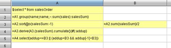
 

esProc Solution

esProc.jpg


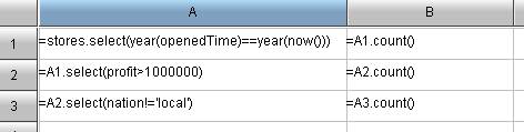
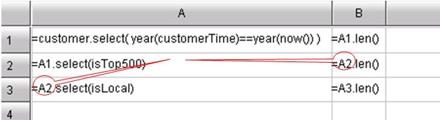
A1 cell: Get the records requested in problem 1.

A2 cell: Step-by-step computation. Operate on the basis of cell A1, and get the record meeting the conditions of problem 2.

A3 cell: Proceed with the step-by-step computation, and get the records requested in the problem 3.

B1, B2, and B3 cell: It is still the step-by-step computation. Count the corresponding records.


Comparison

For the SQL, there are 3 associations for you to compute in steps, and explore progressively. However, because step-by-step computation is hard to implement with SQL, this problem has to be divided into 3 individual problems.


esProc is to compute in steps following the natural habit of thinking: Decompose the general objective into several simple objective; Solve every small objective step by step; and ultimately complete the final objective.


In case that you proceed with the computation on the basis of the original 3problems, for example, seek "proportion of problem 3 taken in the problem 2", or"on" problem 3, group by country". As for esProc users, they can simply write ”=A3/A2”, and ”A3.group(nation)”. In each step, there is a brief and clear expression of highly readable, without any requirements on a strong technical background. By comparison, SQL requires redesigning the statement. The redesigned statement will undoubtedly become more and more complex and longer. Such job can only be left to those who have the advanced technical ability in SQL.


esProc can decompose the complex problem into simple computation procedure based on the descriptions from the business perceptive. This is just the advantage of the step-by-step computation. By comparison, SQL does not allow for computation by step or problem decomposition, and thus it is against the scientific methodology, and not fit for the complex computation.

Complete Set-lization

Case Description

A certain advertisement agency needs to compute the clients whose annual sales values are among the top 10.


The data are from the sales table, which records the annual sales value of each client with the fields like customer, time, and amount.


SQL solution

SELECT customer

FROM (

    SELECT customer

    FROM (

         SELECT customer,RANK() OVER(PARTITION BY time ORDER BY amount DESC) rankorder

         FROM  sales )

    WHERE rankorder<=10)

GROUP BY customer

HAVING COUNT(*)=(SELECT COUNT(DISTINCT time) FROM sales)

Such Problem requires ranking the sets of a set, that is, group by “time” and then rank by “customer” in the group. Since the popular SQL-92 syntax is still hard to represent this, the SQL-2003 standard, which is gradually supported by several vendors, will be used to solve this problem barely.


Just a tip to compute the customer intersections in the last step, the count of years equals to the count of clients.
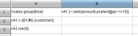
 

esProc Solution

esProc_1.jpg


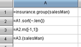
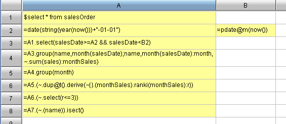
A1: Group the original dataset by year so that A1 will become a set of sets.

B1: Get the serial number of records whose sales values are among the top 10 of each group. The rank() is used to rank in every group, and pselect() can be used to retrieve the serial number on conditions. ~ is used to represent every member in the set. B1 is the “set of set”.

A2: Retrieve the record from A1 according to the serial number stored in B2, and get the customer field of the record.

A3: Compute the intersection of sets.


Comparison


The SQL set-lization is incomplete and can only be used to represent the simple result set. Developers cannot use SQL to represent the concept of “set of set”. Only the queries of 3-level-nested-loops are available to barely perform the similar computations. In addition, SQL cannot be used to perform the intersection operation easily that developers with advanced techniques can only resort to the unreadable statements to perform the similar operations, such as “count of years equal to the count of clients”. It equals to compute the intersection of client sets.

The set is the base of massive data. esProc can achieve set-lization completely, represent the set, member, and other related generic or object reference conveniently, and perform the set operations easily, such as intersection, complement, and union.


When analyzing the set-related data, esProc can greatly reduce the computation complexity. By taking the advantage of set, esProc can solve many problems agilely and easily that are hard to solve with SQL.


III Ordered Set

Case Description

Suppose that a telecommunication equipment manufacturer needs to compute the monthly link relative ratio of sales value (i.e. the increase percent of sales value of each month compared with that of the previous month). The sales data is stored in the sales table with the main fields including salesMonth, and salesAmount.


SQL solution

select salesAmount, salesMonth,

        (case when

prev_price !=0 then ((salesAmount)/prev_price)-1

else 0

end) compValue

from (select salesMonth, salesAmount,

lag(salesAmount,1,0) over(order by salesMonth) prev_price

from sales) t


The popular SQL-92 has not introduced the concept of serial number, which adds many difficulties to the computation. Considering this, the designer of SQL-2003 has partly remedied this drawback. For example, the window function lag() is used to retrieve the next record in this example.

In addition, in the above statement, the “case when” statement is used to avoid the error of division by zero on the first record.


esProc Solution

  1. sales.derive(salesAmount / salesAmount [-1]-1: compValue)


The derive() is an esProc function to insert the newly computed column to the existing data. The new column is compValue by name, and the algorithm is “(Sales value of this month/Sales value of previous month)-1”. The “[n]” is used to indicate the relative position, and so [-1] is to represent the data of the previous month.


On the other hand, for the data of the first record, the additional procedure for division by zero is not required in esProc.


Comparison

From the above example, even if using SQL-2003, the solution to such problem is lengthy and complex, while the esProc solution is simple and clear owing to its support for the ordered set.


Moreover, SQL-2003 only provides the extremely limited computation capability. For example, esProc user can simply use the ”{startPosition,endPosition}” to represent the seeking of a range, and simply use ”(-1)” to represent the seeking of the last record. Regarding the similar functionality, it will be much harder for SQL user to implement.


In the practical data analysis, a great many of complex computations are related to the order of data. SQL users are unable to handle such type of computations as easily as esProc users because SQL lacks of the concept of Being Ordered.


IV Object Reference

An insurance enterprise has the below analysis demands: to pick out the annual outstanding employees (Employee of the Year) whose Department Manager has been awarded with the President Honor. The data are distributed in two tables: department table (main fields are deptName, and manager), and employee table (main fields are empName, empHonor, and empDept).


empHonor has three types of values: null value; ”president's award”, PA for short; and ”employee of the year”, EOY for short. There are 2 groups of correspondence relations: empDept and deptName, and Manager and empName.


SQL solution

SELECT A.*

FROM employee A,department B,employee C

WHERE A.empDept=B.deptName AND B.manager=C.empName AND A.empHonor=EOY AND C.empHornor=PA


SQL users can use the nested query or associated query to solve such kind of problems. In this case, we choose the association query that is both concise and clear. The association statement behind the “where” has established the one-to-many relation between deptName and empDept, and the one-to-one relation between manager and empName.


esProc Solution


   employee.select(empHonor:"EOY",empDept.manager.empHornor:"PA")


esProc solution is intuitive: select the employee of “EOY” whose Department Manager has be awarded with “PA”.


Comparison

The SQL statement to solve such kind of question is lengthy and not intuitive. In fact, the complete association query language is “inner join…on…” style. This statement is simplified in the above example. Otherwise it will be much hard to understand.


esProc users can use ”.” for object reference. Such style is intuitive and easy to understand. The complex and lengthy association statement for multiple tables can thus be converted to the simple object access, which is unachievable for SQL. When there are more and more tables, the complexity of SQL association query will rise in geometric series. By comparison, the esProc user can always access the data intuitively and easily by taking the advantage of object reference.


Regarding the multi-table associations of complex computation, esProc can handle it more intuitively and conveniently than SQL.

From the comparison of the above four examples, we can see that esProc is not only characterized with step-by-step computation, complete set-lization, sorted sets, and object reference. The analysis style is intuitive, the syntax style is agile, and the function is powerful. esProc is a tool especially designed for mass data computation, and a more convenient database computing script.
About esProc: http://www.raqsoft.com/product-esproc

raqsoft

Tap Utmost Value of Excel

Posted by raqsoft Apr 10, 2014

Excel is the most widely-used spreadsheet tool. The nontechnical persons love to use it for computation and analysis though, they usually find the formulas and functions available in Excel are rather poor and the VBA is just double Dutch to them for further analysis. Thus, a huge volume of data with valuable information has been wasted in vain.


esProc is introduced to better the situation. Empowered esProc users can tap the utmost value of Excel by taking the esProc advantages of powerful computation ability, agile and easy-to-use analysis style, and programmed running mode.


I Case and Comparison

Description

In an advisement agency, a Sales Director receives Client Reports from eight Regional Account Managers by every quarter. The Client Report is an Excel spreadsheet, mainly comprising the client, sales value, and other information about the respective region, as given in the below figure: 

esProc.png


Suppose that the Sales Director wants to compare the big client across various regions. For example, regarding the client of whom the sales value ranks top 10%, 20% or 30%, what’s the average sales, and which enterprise is among the Top 500?


First, let’s have a look at the attempt to solve it with Excel formulas.

Excel Formula Solution


The first step is to compute the average sales of clients whose sales values rank top 10%. We may adopt the following procedure: firstly, sort the sales value in descending order, and then use count( ) function to compute the total number of clients. Secondly, multiple the total number by 10%, and round the result to get the row number with the round ( ) function. Finally, copy these clients onto a new spreadsheet, and compute the average value. This procedure is not difficult for those who are familiar with Excel.


Then, let’s proceed with this computation: How many of these big clients are among Top 500? To solve the problem, you need to get the intersection of the two datasets. In other words, this is to compute the common part of big client set and the Top 500 list from the previous step. The computational expression is:

=INDEX(A:A,SMALL(IF(COUNTIF($B$2:$B$15,$A$2:$A$20),ROW($A$2:$A$20),4^8),ROW(A1)))&"


Since the above formula requires 5 various combinations of functions, it is a great challenge to compose it.


To make it worse, the computational procedure of Excel requires the user to carry out manually and only acceptable for the specific Excel spreadsheet. This is not as universal as a program, for example, if program, the whole computational procedure will rerun automatically on receiving different file names. In this case, there are 8 Excel® files. Excel users will have to run the computational procedures for 8 times. Moreover, there are 3 rankings: 10%, 20%, and 30%, which means the computation will have to be repeated for 8X3=24 times.


It is obvious that it is too tough to solve this problem with Excel formula.


Let’s try VBA, the most powerful extension tool of Excel.


Excel VBA® Solution

Function Collection(a As Range, b As Range)

On Error Resume Next

    Dim arr1(), arr2(), times, tmpindex

    Set newcoll = CreateObject("Scripting.Dictionary")

    With Application.WorksheetFunction

        arr1 = .Transpose(a.Value)

        arr2 = .Transpose(b.Value)

        Do

            times = .Mode(arr1, arr2)

            If IsEmpty(times) Then

                Exit Do

            Else

                newcoll.Add times, Empty

                tmpindex = .Match(times, arr1, 0)

                arr1(tmpindex) = arr1(UBound(arr1))

                If UBound(arr1) = 1 Then

                    arr1(1) = Empty

                Else

                    ReDim Preserve arr1(1 To UBound(arr1) - 1)

                End If

                tmpindex = .Match(times, arr2, 0)

                arr2(tmpindex) = arr2(UBound(arr2))

                If UBound(arr2) = 1 Then

                    arr2(1) = Empty

                Else

                    ReDim Preserve arr2(1 To UBound(arr2) - 1)

                End If

                times = Empty

            End If

        Loop

    End With

    arr3 = newcoll.keys

    If newcoll.Count = 0 Then

             Collection = False

    Else

             Collection = arr3

End If

End Function


Isn’t it unreadable and indigestible? The above “double Dutch” is only one step to compute the intersection set of several steps. Undoubtedly, VBA needs a great programming capability and is by no means suitable for nontechnical persons.

Then, let’s check the impressive esProc solution below.


esProc Solution

esProc_2.png

A1 and A6: Retrieve the “Client Report” of a certain region respectively and “Top 500 list”. Please note that “rangeFile” is a parameter, and you can assign various file names to get various results. In addition, the “percent” in the B2 is also a parameter, for example, 10%, 20%, and 30%.

A2: Sort the data in A1 by sales value. The ”amount” is column name retrieved automatically, and the ”-1” represents the descending order.

B2: Compute the row number of clients ranking the top 10%, 20% or 30% respectively.

A3: Compute the clients from row 1 to B2 that are all big clients. Assume that B2 equals to 3, then “to(B2)” equals to ”1,2,3”.

A4: Compute the average sales value of big clients

A7: Compute the clients which not only big clients but also among the Top 500. In other words, this is to compute the intersection set of the customer column from the Client Report and the 500Name column from the Top 500. The ”^” represents the intersecting action.

A8: Compute the number of clients in the intersection set from the previous step.

As we can see, the style of esProc expression is similar to that of Excel®, agile and intuitive but more powerful in computing and capable to rerun just as a program does. It is a great analysis tool to empower the nontechnical persons who are familiar the style of Excel®.

Perfect! esProc is just the best tool to solve such problems.

II Features Fit for Excel

Better Usability

esProc provides an operation interface of “cellset” style with the letter as column name and number as row no. The cells can be mutually referenced with cell name. Such style is quite friendly to people who are familiar with Excel.

The cellset allows the business analyst to work from the business perspective, process and analyze the data intuitively. Therefore, esProc demands little on technical capability from users, and thus ideal for business person with no technical background.

esProc can be installed on the normal PC with common OS , and run in a environment similar to that of Excel.


Strong Analysis Ability

As a tool specially designed to handle massive data computations, esProc has all capability of SQL statements and senior languages. On one hand, esProc can be used to query, filter, group, and collect statistics, just like SQL statements; On the other hand, it can be used in the loop and branch judgment for the procedure analysis, just like VBA.

In the practical use, esProc over-performs the SQL and senior languages, thanks should go to the below advantages: esProc users will never face the dilemma of lengthy and unreadable SQL statements and the poor computability of senior languages. Even the nontechnical person can also resort to esProc to complete the complex analysis computation all by themselves.


Programmed Running Mode

esProc has special optimizations for Excel, providing the easy-to-use functions for reading from or writing back to Excel® spreadsheets of various versions from Excel®97 to Excel®2007.

In a programmed running mode, esProc users can analyze various Excel® spreadsheets according to various parameters, which is ideal for the repetitive computation. It is indeed a timesaving and effort-saving analysis tool.


III Significance and Value to Excel

esProc is a powerful analysis tool for Excel, and particularly suits the need of nontechnical persons to implement complex computational analysis on data from Excel® spreadsheets.


esProc facilitates the data mining on Excel with the convenience and power for all people to deliver and ensure the valuable data will truly support the decision-making of enterprises.


esProc saves the long-stored Excel® from turning into a legacy over time. esProc will tap the utmost value of Excel.


About esProc: www.raqsoft.com/product-esproc

In Java, implementing via SQL is a well-developed practice for database computing. However, the structured data is not only stored in the database, but also in the text, Excel, and XML files. Considering this, how to compute appropriately regarding the structured data from non-database files? This article raises 3 solutions for your reference: implement via Java API, convert to database computation, and adopt the common data computation layers.


Implement via Java API. This is the most straightforward method. Programmers will benefit from Java API in controlling every computational step meticulously, monitoring the computed result in each step intuitively, and debugging conveniently. Needless to say, no learning cost is also an additional advantage of Java API.


Thanks to the well-developed API for retrieving and writing-back data to Txt, Excel, and XML files, Java has enough technical strength to offer the full support for such computation, in particular the simple computational goals.


However, this method requires great workload and quite inconvenient.


For example, since the common data algorithms have not implemented in Java, programmers will have to spend great time and efforts to implement all the ins and outs manually by aggregating, filtering, grouping, and sorting and some other common actions.


For another example of data storage and detail data retrieval through Java API, programmers will have to combine every data and 2D table with List/map and other objects, and then compute in nested loops at multi-levels. Moreover, such computation usually involves the set operations and relational computations on massive data, as well as the computations between objects and object properties. It takes great efforts to implement the underlying logics and even greater workload in handling the complex ordered computation.


In order to reduce the programming workload, programmers always prefer leveraging the existing algorithms to implementing all specifics by themselves. In view of this, the second choice below would be a better choice:


Convert to database computation. This is the most conservative method. Concretely speaking, it is to import the non-database data to the database via the common ETL tools like DataStage, DTS, Informatica, and Kettle. The advantages of this practice include the high computational efficiency, steadfast running, and less workload for Java programmers. It fits for the scenarios of great data volume, high performance demand, and medium-level computational complexity. These advantages are evident for the mixed computation on the database and the non-database files in particular.


The main drawback of this method is the great workload in the early stage of ETL and the great maintenance difficulty. First, since the non-database data cannot be used directly without field-splitting, merging, and judging, programmers have to write a great many of Perl/JS scripts to clean and re-organize the data. Second, the data is usually updatable, so the scripting must handle the changing incremental update issues. The data from various data sources can hardly be compatible with a normal form. So, the data is unusable before the level 2 or even the level 3 ETL process. Third, scheduling is also a problem when there are lots of tables – which table must be uploaded first? Which one is the second to upload? What’s the interval? In facts, the huge workload of ETL is always beyond our expectation, and it is always quite tough to evade project risk. Plus, the real-time performance of ETL is poor owing to the regular transit of the database.


In some operating environments, there is probably no database service at all for the sake of security or performance. For another example, if most data is saved in the TXT/XML/Excel and no database involved, then the existence value of ETL gets void. What can we do? Let’s try the 3rd method:


The common data computational layer is typified by the esProc and R. The data computational layer is a layer in-between the data persistence layer and the application layer. This layer is responsible for computing the data from data persistence layer uniformly and returning the computed result to the application layer. The data computation layer of Java is mainly used to reduce the coupling between the application layer and the data persistence layer, and alleviate the computational pressure on them.


The common data computational layer offers the direct support for various data sources - not only the database, but also the non-database data sources. By taking the advantage, programmers can access to various data sources directly, free from such things as real-time problems. In addition, programmers are allowed to implement the interactive computation between various data sources conveniently, for example, the computations between DB2 and Oracle, and MYSQL and Excel. In the past, such access is by no means easy to implement.


The versatile data computational layers are usually more professional on structured data, for example, it supports the generic, explicit set, and ordered array. So, the complex computational goals, which are tough jobs for ETL/SQL and other conventional tools, can be solved with this layer easily.


The drawback of such method mainly lies in the performance. The common data computation layer is of the full memory computation, so the size of memory determines the upper limit of the data volumes to handle. But both esProc and R support the Hadoop directly so that their users can handle the big data in the distributed environment.


The main difference between esProc and R is that esProc supports the direct JDBC output and convenient integrating with Java codes. In addition, esProc IDE is much easier to use, with the support for the true debugging, and scripts in grid, and cell name for direct referencing the computed result. R does not provide such advantages, nor support for JDBC, and thus a bit complex for R users to integrate. However, R supports the correlation analyses and other model analyses. R programmers do not have to implement all specifics to generate the computed result directly. R also supports the Txt/ Excel / XML files and other lots of more non-database data sources. By comparison, esProc only supports 2 of them. The last but not the least advantage of R is that the low-end edition of R supports the open source to the full.


The above is the comparison between these three methods, and you can choose the right one based on your project characteristics.


Web: http://www.raqsoft.com/product-esproc

In the previous article, I’ve shared some experiences in Hadoop coding with the agile esProc syntax. This article is the supplementary and in-depth discussion based on the previous one.


Firstly, let’t talk about the Cellset Code.


In the previous article, I ‘ve introduced the convenience of using cellset code to define variable, make reference to variable, and achieve the complex computation goal in multiple steps. In facts, the cellset or grid can be used to make it more simple to reuse the computational result. Please refer to the code block below:

esProc1.jpg


As can be seen, the computational result in A2 is reused in B2 and A3.


The introduction of grid line in the cellset is a good idea. The grid line can keep the code lines aligned naturally, for example, form a clear and intuitive work scope by indentation. Take the below code for example:

esProc2.jpg


Look good. The branch of judgment statement can be recognized well. The code block appears clear and neat without the deliberate edits.


Then, let’s talk about the Object Reference. What is the object reference? Take a previous code snippet for example: A10: =A9. sort(sumAmount: -1). select(#<=10),


The code in A10 can be rewritten in two cells separately, one for sorting, and another for filtering. But in the actual given code, the “,” is used to consolidate the computations of these two steps - this mechanism is referred to as the Object Reference. Object Reference reduces the workload of coding and result in the more agile coding.


Support for direct writing the SQL Statement

The big data computing usually involves the access to Hive database or traditional database. MapReduce requires users to write the complex connect\statement\result statement, while esProc supports direct composing the SQL statement to saves users all these troubles. For example, to get the sales record from the the data source HData of a Hive database, esProc enables users to complete all work with one statement: $(HData)select * from sales.


Function options

Firstly, let’s check out these two statements in the sample code from the first article:

? Code for node machine A2: =A1. groups(${gruopField};${method}(${sumField}): Amount)

? Code for summary machine A9: =A8. groups@o(${gruopField};${method}(Amount): sumAmount)

The former one uses the groups directly to group the unsorted data. The latter one uses the @o option to indicate that the sorted data have been grouped for a much higher speed. @o is a function option to reduce the complex function of heavy workload and make it easier to memorize the names of various functions to achieve different functions. In addition to @o, there are @m and @n function options of the groups function


The function option is a nice design to make the function structure much simpler, and the coding more agile.


Multi-level Parameter

The multi-level parameter (or hierarchy parameter by name) can make the syntax much agile. This is a way to represent the parameters at different levels of the function, for example, ranking the employee by its performance score:

? If the performance score is higher than 90, then set it to “A”

? If the performance score is between 90 and 60, then set it to “B”

? If the performance score is between 60 and 30, then set it to “C”

? If the performance score is below 30, then set it to “D”

In the esProc, the above parameters can be represented like this: score>90:" A",score>60 && score< 90:" B",score>30 && score<=60:" C";"D"


In this case, the parameter can be classified into three levels, and the outermost level: The branch and the default branch is separated with “;”; The middle level: Each branch is separated with “,”; The innermost level: The judgment expressions and results in each branch are separated with “: “. This is a parameter combination of three-level tree structure.


Set-style Grouping

esProc supports the set-style grouping, and is also capable of coding in an agile way. The essence of dynamic data type is the set. Specifically, the simple data type is the set of single value, the array is the set of alike data, and the two dimensional table is the set of records. The member of a set can be another set. Therefore, esProc can be used to represent the concept of grouping in the data computation: Each group is a member of a set, and the member itself is a set. Thanks to the agile syntax, the set-style grouping can be used to solve the complex grouping and computational problems. For example, find the sales person who signed the most and the least insurance policies. The code is as shown below:

esProc3.jpg

A1 cell: Group by sales person. Each group is a set of all policies of one sales person.

A2 cell: Sort the group by the number of policies. In the code snippet, the “~” represents a group of policies corresponding to each sales person.

A3 cell: Find the groups having the most or the least polices. They are the first group and the last group in cell A2.

A4 cell: List the name of sales person. They are the sales persons corresponding to the two groups of policies in A3.


The agile syntax of esProc boosts the efficiency of code development, and reduces the development workload dramatically.


Web: http://www.raqsoft.com/product-esproc

The columnar storage is good, especially when there are lots of tabular fields (this is quite common). In querying, the data to traverse is far less than that on the row storage. Less data to traverse brings less I/O workloads and higher query speed. However, the Hadoop application consumes most time on the hard disk I/O without columnar storage.

Both Hive and Impala support columnar storage, but columnar storage only available with the basic SQL interface. As for some more complex data computing, it seems quite difficult for the MapReduce framework to do columnar storage.

The sample data is a big data file sales.txt on the HDFS. This file has twenty fields, 100 million data entries, and the file size is 14G. Let’s take the GROUP computing for example to demonstrate the whole procedure. Concretely speaking, it is to summarize the total sales for everyone by the sales person. The algorithm involves two fields, empID and amount.

Firstly, compare it with the classic code for Grouping and Summarizing on Columnar Storage:

Code for summary machine:

columnar_storage.png

Code for node machine:

columnar_storage_2.png

The above columnar storage algorithm follows such train of thought: Scheduling a large task into forty smaller tasks according to the file bytes; distribute them to the node machine for the initial summarization; and then further secondary summarize on the summary machine. This train of thoughts is similar to that for MapReduce. The difference is that this columnar storage thinking pattern is simple and intuitive because the task scale could be customized, and most people can understand it easily.

As can be seen, the row storage is to store all fields in the file in the form of fields. Therefore, no matter there are two or twenty fields, we still have to traverse all data – the file of 14 G. However, the columnar storage is not like this. The data of each field are stored as a file. If only two fields are stored in the query, then you only need to retrieve the corresponding file of these two fields, i.e. 1.4 G. Please note that the 1.4 G is an average value. The total volume of the data of the two fields is slightly higher than 1.4 G.

As mentioned above, to implement the columnar storage, we must decompose the file field by field first, by using f.cursor() to retrieve first and then f.export() to export. The detailed procedure about columnar storage will be explained at the end of this article.

Code for Grouping and summarizing once Columnar Storage is adopted:

Code for summary machine:

columnar_storage_3.jpg

Code for node machine:

columnar_storage_4.png

As can be seen, the greatest change is the code for node machine. The A3 cell uses the [file list]. Use the cursor() to merge a group of field files to generate a cursor of 2 dimension table. The remaining codes for grouping and summarizing are just the same as before.

Another change is about the task-scheduling. In fact, great trouble can be caused in this stage. As we know, in the row storage, the task-scheduling can be performed based on the number of byes. For example, a 14 G file can be divided into 40 segments evenly, and each segment will be assigned to a node machine as a task. But this method does not work in the columnar storage because of the record misalignment, and the result can be always wrong. The right method is to divide evenly by the number of records (Any suggestions on dividing it evenly, please leave a comment. Thanks.). 100 million entries can be allocated to 40 segments, and each segment will hold 2’500’000 entries.

For example, the empID column will be ultimately divided into 40 smaller files: empID1. dat”,”empID2. dat”……”empID40. dat”. Then, the algorithm codes are shown below:

columnar_storage_5.jpg

In order to prevent the memory overflow, the above algorithm will retrieve 100’000 entries from cursor, and append to the file. By doing this, a new file will be created with every 2’500’000 entries of data. In which, A3 is the file count, C3 is used to monitor if the data entries in the current files reaches 2.5 M.

The data-scheduling is surprisingly troublesome, but the columnar computing after splitting is quite simple.

Web: http://www.raqsoft.com/

raqsoft

6 Data Computing Tools

Posted by raqsoft Jan 23, 2014

Recently, I finished a project which involves using the Excel, R Project, and es-series in combination. An idea occurred to me in the work. Why not put them along with the Matlab, SPSS, and Stata side-by-side to make an introductions and comparisons of Desktop BI tools? At last, this essay comes into being, as you can see below.

Desktop BI refers to the BI tools running on the desktop environment, almost not requiring any server supports. The typical Desktop BI only provides the core BI functions with less requirement on the technical environments. By comparison, such software as Solution BI cannot operate without the support from private server. They are usually the integrated solution or platform system in-built with lots of half-finished components. Besides the core BI functions, Solution BI also provide some non-core functions like the authority management, resources sharing, and collaboration between jobs of various types. Desktop BI is the commonest tool for people doing the data computing and analysis.

Comparison results:

Technical Requirements:              Excel > ES Series> SPSS >Matlab >STATA >R

Numbers of statistical models:   R >STATA >SPSS >Matlab >Excel >ES Series

API capability:           R >Excel > STATA > Matlab >SPSS >ES Series

Complex computing goal:      ES Series  >R >Matlab >Excel >STATA >SPSS

Graphic capability:                  SPSS >R > Matlab  > ES Series  >Stata >Excel

Learning curve:              Excel > SPSS > ES Series >Matlab >STATA >R

Interactive computing:      ES Series  > Excel  >R >Matlab >STATA >SPSS

Price:                         R >Excel >ES Series >Stata >Matlab >SPSS

Note: In the above comparison, the tool on the left has more advantages than those the right.

Excel

Of all BI software, which one occupies the largest market shares, has the largest user base, and experiences the greatest increase in each year? It is neither QlikView / Spotfire, nor SAS / SAP, but Excel. Does it surprise you? BI producers are always running down Excel in an attempt to describe Excel as “inferior BI toy” or even “outdating BI”. But the figures won’t lie, Gartner, many true BI users, and even these producers have to admit that Excel is the most (not just the one of the most) important BI tool.

Excel is an intuitive and flexible Desktop BI tool of low technical threshold. BI is aimed to solve the “Business” problem. Who understand the business best? Needless to say, it is the business experts – the core users of BI software. Most of them do not have strong technical background, so they wish the technical threshold will be as low as possible. It seems Excel lack the computing capability and it is hard for Excel to handle the abstract data structure as the SQL and other script languages do. However, confronting the intuitive data directly, Excel has the advantage of providing a flexible and natural computing method. The business experts can be benefited to turn their business algorithm into computer languages according to their business thoughts. This is great expression ability of BI tools. Although other BI tools are more powerful in computing, they are too difficult for business experts to use in expressing the business algorithms. Therefore, no matter how powerful computing capability these tools have got, the business experts cannot leverage it.

R Project      http://www.r-project.org/

R Project holds the largest market shares of open source BI tools. In the KDNuggets survey 2012 on the “Top Analytics, Data Mining, and Big Data software used”, R won the top one title with 30.7% of votes. It is often used for the statistical analysis, matrix computing, and graphic plotting, mainly in the sector of information biology and partly in the economic measurement, financial analysis, and cultural sciences.

R features the interactive computing environment and the abundant 3rd party library functions. R offers an intuitive way to view and make reference to the results of previous computing. Relying on the agile and elegant syntax, R users can carry forward the data processing step by step, and decompose the complex computing goal into several simple goals easily. Such interactive computing environment is ideal for solving the complex and ambiguous BI problems. R is the open-source software with massive function libraries and rapidly updating algorithms. Its secondary development interface supports various languages for users to integrate the 3rd party library functions easily, so it becomes widely popular with a great many users.

Comparatively, R suffers some drawbacks on UI friendliness and technical requirements, which hinders R from further popularization. RStudio and the alike tools can remedy the weak points of R on UI friendliness. However, it is still a far cry from the business software, and the technical requirement on languages is native and unchangeable. Moreover, many people also complain on the relatively low computing speed and the unsatisfactory accuracy of package from the 3rd party.

Last, thanks to the powerful computing capability and the open source characteristic of R, various big data solutions like Teradata , SAP, Oracle, and IBM all declared their support for R and R thus holds the spotlight.

ES Series      http://www.raqsoft.com

ES Series is the next generation Desktop BI tool of the most promising one in making a breakthrough on the traditional BI. Regarding the spreadsheets sector, es-series provides a more powerful computing capability than Excel, quite suitable for the business personnel without technical background to conduct the complex data computing. It implements the homocell model and the visualization of computing procedure. es-series not only allows for the intelligent formula-pasting to reduce the manual operations dramatically and the free step-by-step computing to implement the free data manipulation, but also provides the all-around set computing ability to solve the complex computing easily. The users of es-series tools can perform the table association operation to implement the computing between multiple tables with none formula required. These advantages are always the bottlenecks for the traditional spreadsheets.

Regarding the data computing scripts, es-series tools have the same complete structural data computing ability as SQL, with much lower technical requirements. es-series tools are the same capable as R in its interactive computing abilities to solve the complex problems, and offer a friendlier interface. The syntax of es-series is more intuitive and easier-to-understand. It is the computing scripts that business personnel can grasp easily. Considering its distinguishing features, es-series is superior to SQL or R on many respects. For example, es-series can reach the complex goal of computing more easily through the step-by-step computing in the cellset; its support for explicit sets allows for the intuitive data manipulation from business perspective, and will ultimately reduce the difficulty and improve the readability; es-series tools enable the object reference to implement the associative access to multi-tables intuitively, and support the sorted set to solve any tough problems related to orders.

However, es-series tools comparatively lack such model algorithm as regression analysis, collaboration, and sharing that Excel provides.

SPSS      http://www-01.ibm.com/software/analytics/spss/

SPSS is reputed for its simplicity and friendliness and occupies the greatest market share. SPSS provides the completely graphical UI for operations and the command options of menu style, so that users can perform the commonest module analysis without any scripting. With regard to the fixed module analysis, SPSS is really good at the ANOVA and Multivariate Statistical Analysis. They even do better than SAS of Solution BI in this aspect.

The overall ability in graphic drawing of SPSS is the best among all Desktop BI software. Although the drawing plotted by R is also quite fine, the interactive plotting procedure of SRSS can overtake R completely. Almost everything in the drawings can be altered. No matter it is the statistic chart design stage or the graphic result stage, users can directly alter the colors and line patterns. They can also add the marking variables in the Scatter Diagram or even change the 2D to 3D, or delete some data, or change the basic type of drawings, for example, change the bar charts to the line charts, and add several auxiliary lines at will. Drawing with SPSS will give you a feeling of acting willfully.

However, SPSS is comparatively rather rigid, and only capable to perform the analysis on fixed model. It is quite hard for SPSS users to perform the computing outside the models. For example, firstly, filter the analysis result by the keyword; then rank by another column; secondly, retrieve the several top rankings; and lastly convert the unit of values in a certain column from US Dollar to the Pound. In this aspect, it is quite natural that the computing scripts of R, esProc, and MATLAB are more powerful. Therefore, SPSS cannot be used for free computing and complex analysis. It is the fool-proof software. In addition, SPSS is quite expensive. STATA is comparatively more cost-effective.

STATA    http://www.stata.com

STATA can be regarded as the tools between SPSS and R, considering the price, interface friendliness, flexibility, and degree of freedom. Almost all SPSS fixed analysis models have the corresponding features in STATA. The differences are that SPSS provides the friendly parameter-inputting interface and result representation interface for analysis, while STATA only provides the command line prompt for input and console text output. In addition, the regression analysis of STATA is more powerful than several other tools, such as OLS. The similar advantageous analyses include the Time series analysis and the Panel Data analysis.

The drawing ability of STATA is also fine and almost at the same level as that of es-series and R, although it is worse than that of SPSS.

I disagree to the opinion held by some people that STATA is the commercialized R. Although the expansibility of STATA is greater than that of SPSS, and the 3rd party vendors can update the algorithm timely, it is still far worse than that of R. In addition, R, es-series, and MATLAB are the most typical computing scripts, which allow for the free analysis in a way similar to programming. By comparison, STATA is a bit rigid and awkward. We can reach this conclusion:

R can provide all features of STATA, while STATA may not have some features of R. SPSS cannot give the desired features for it doesn’t have, STATA can give them in a very awkward and rigid way, R can give them normally, while esProc can give them easily.

MATLAB  http:// www.mathworks.com/products/matlab/

MATLAB is a computing language and interactive environment for numerical calculation, algorithm development, and data analysis, enabling users to create the user interface by plotting the graphic for themselves. Matlab is widely applied in the industrial automation system design and analysis, as well as the sectors of graphic processing, signal processing, communications, finance-modeling & analysis.

At a first glance, it appears that Matlab and R shares many similarities in the UI style, syntax structure, graphic capability, and other aspect. Their differences are great. Matlab is the shortened form of Matrix Laboratory. As the name implies, it is the best at the matrix computation. Matlab can provide more mathematical functions than R. In addition, it can provide many functions based on in-depth study on the specific industries or majors, for example, industrial data analysis, financial model setup, and neural network toolbox. Matlab can do more professionally in these areas than R. Its graphical operation capability is greater than that of R but worse than that of SPSS.

Comparatively, R has stronger language expressing ability and more powerful statistic functions than Matlab. In other words, R is simpler and more flexible to convert the algorithms on paper to the languages that computers could understand. In addition, the statistical module of Matlab is neither complete nor updated.

As to the price of MATLAB, its price is between SPSS and STATA, which is “a little expensive”.

Conventionally, we shall say that each of these tools has its strong point and let’s use them in combination. But according to my years of experiences, I would like to offer an personal advice that the tool capable of expressing your thoughts freely is the tool best for you.

Web: http://www.raqsoft.com/

Hadoop is an outstanding parallel computing system whose default parallel computing mode is MapReduce. However, such parallel computing is not specially designed for parallel data computing. Plus, it is not an agile parallel computing program language, the coding efficiency for data computing is relatively low, and this parallel computing is even more difficult to compose the universal algorithm.


Regarding the agile program language and parallel computing, esProc and MapReduce are very similar in function.


Here is an example illustrating how to develop parallel computing in Hadoop with an agile program language. Take the common Group algorithm in MapReduce for example: According to the order data on HDFS, sum up the sales amount of sales person, and seek the top N salesman. In the example code of agile program language, the big data file fileName, fields-to-group groupField, fileds-to-summarizing sumField, syntax-for-summarizing method, and the top-N-list topN are all parameters. In esProc, the corresponding agile program language codes are shown below:


Agile program language code for summary machine:

Agile program language code for node machine:


How to perform the parallel data computing over big data? The most intuitive idea occurs to you would be: Decompose a task into several parallel segments to conduct parallel computing; distribute them to the unit machine to summarize initially; and then further summarize the summary machine for the second time.


From the above codes, we can see that esProc has parallel data computing into two categories: The respective codes for summary machine and node machine. The summary machine is responsible for task scheduling, distributing the task to every parallel computing node in the form of parameter to conduct parallel computing, and ultimately consolidating and summarizing the parallel computing results from parallel computing node machines. The node machines are used to get a segment of the whole data piece as specified by parameters, and then group and summarize the data of this segment.


Then, let’s discuss the above-mentioned parallel data computingcodes in details.

Variable definition in parallel computing


As can be seen from the above parallel computing codes, esProc is the codes written in the cells. Each cell is represented with a unique combination of row ID and column ID. The variable is the cell name requiring no definition, for example, in the summary machine code:

n  A2: =40

n  A6: = ["192. 168. 1. 200: 8281","192. 168. 1. 201: 8281","192. 168. 1. 202: 8281","192. 168. 1. 203: 8281"]

A2 and A6 are just two variables representing the number of parallel computing tasks and the list of node machines respectively. The other agile program language codes can reference the variables with the cell name directly. For example, the A3, A4, and A5 all reference A2, and A7 references A6.


Since the variable is itself the cell name, the reference between cells is intuitive and convenient. Obviously, this parallel computing method allows for decomposing a great goal into several simple parallel computing steps, and achieving the ultimate goal by invoking progressively between steps. In the above codes: A8 makes references to A7, A9 references the A8, and A9 references A10. Each step is aimed to solve a small problem in parallel computing. Step by step, the parallel computing goal of this example is ultimately solved.


External parameter in parallel computing


In esProc, a parameter can be used as the normal parameter or macro. For example, in the agile program language code of summary machine, the fileName, groupField, sumField, and method are all external parameters:

n  A1: =file(fileName). size()

n  A7: =callx(“groupSub. dfx”,A5,A4,fileName,groupField,sumField,method;A6)

         They respectively have the below meanings:

n  filename, the name of big data file, for example, " hdfs: //192. 168. 1. 10/sales. txt"

n  groupField, fields to group, for example: empID

n  sumField, fields to summarize, for example: amount

n  parallel computing method, method for summarizing, for example: sum, min, max, and etc.

If enclosing parameter with ${}, then this enclosed parameter can be used as macro, for example, the piece of agile program language code from summary machine

n  A8: =A7. merge(${gruopField})   

n  A9: =A8. groups@o(${gruopField};${method}(Amount): sumAmount)

In this case, the macro will be interpreted as code by esProc to execute, instead of the normal parameters. The translated parallel computing codes can be:

n  A8: =A7. merge(empID)   

n  A9: =A8. groups@o(empID;sum(Amount): sumAmount)


Macro is one of the dynamic agile program languages. Compared with parameters, macro can be used directly in data computing as codes in a much more flexible way, and reused very easily.


Two-dimensional table in A10

Why A10 deserves special discussion? It is because A10 is a two-dimensional table. This type of tables is frequently used in our parallel data computing. There are two columns, representing the character string type and float type respectively. Its structure is like this:

         empID

sumAmount

C010010

456734. 12

C010211

443123. 15

C120038

421348. 41


In this parallel computing solution, the application of two-dimensional table itself indicates that esProc supports the dynamic data type. In other words, we can organize various types of data to one variable, not having to make any extra effort to specify it. The dynamic data type not only saves the effort of defining the data type, but is also convenient for its strong ability in expressing. In using the above two-dimensional table, you may find that using the dynamic data type for big data parallel computing would be more convenient.


Besides the two-dimensional table, the dynamic data type can also be array, for example, A3: =to(A2), A3 is an array whose value is [1,2,3…. . 40]. Needless to say, the simple values are more acceptable. I’ve verified the data of date, string, and integer types.


The dynamic data type must support the nested data structure. For example, the first member of array is a member, the second member is an array, and the third member is a two-dimensional table. This makes the dynamic data type ever more flexible.


Parallel computing functions for big data

In esProc, there are many functions that are aimed for the big data parallel computing, for example, the A3 in the above-mentioned codes: =to(A2), then it generates an array [1,2,3…. . 40].


Regarding this array, you can directly compute over each of its members without the loop statements, for example, A4: =A3. (long(~*A1/A2)). In this formula, the current member of A3 (represented with “~”) will be multiplied with A1, and then divided by A2. Suppose A1=20000000, then the computing result of A4 would be like this: [50000, 100000, 1500000, 2000000… 20000000]


The official name of such function is loop function, which is designed to make the agile program language more agile by reducing the loop statements.


The loop functions can be used to handle whatsoever big data parallel computing; even the two-dimensional tables from the database are also acceptable. For example, A8, A9, A10 - they are loop functions acting on the two dimensional table:

n  A8: =A7. merge(${gruopField})    

n  A9: =A8. groups@o(${gruopField};${method}(Amount): sumAmount)

n  A10: =A9. sort(sumAmount: -1). select(#<=10)


Parameters in the loop function

Check out the codes in A10: =A9. sort(sumAmount: -1). select(#<=10)


sort(sumAmount: -1) indicates to sort in reverse order by the sumAmount field of the two-dimensional table of A9. select(#<=10) indicates to filter the previous result of sorting, and filter out the records whose serial numbers (represented with #) are not greater than 10.


The parameters of these two parallel computing functions are not the fixed parameter value but parallel computing method. They can be formulas or functions. The usage of such parallel computing parameter is the parameter formula.


As can be seen here, the parameter formula is also more agile syntax program language. It makes the usage of parameters more flexible. The function calling is more convenient, and the workload of coding can be greatly reduced because of its parallel computing mechanism.


From the above example, we can see that esProc can be used to write Hadoop with an agile program language with parallel computing. By doing so, the code maintenance cost is greatly reduced, and the code reuse and data migration would be ever more convenient and better performance with parallel computing mechanism.


Personal blog: http://datakeyword.blogspot.com/

Web: http://www.raqsoft.com/

The MapReduce of Hadoop is a widely-used parallel computing framework. However, its code reuse mechanism is inconvenient, and it is quite cumbersome to pass parameters. Far different from our usual experience of calling the library function easily, I found both the coder and the caller must bear a sizable amount of precautions in mind when writing even a short pieces of program for calling by others.


However, we finally find that esProc could easily realize code reuse in hadoop.   Still a simple and understandable example of grouping and summarizing, let’s check out a solution with not so great reusability. Suppose we need to group the big data of order (sales.txt) on HDFS by salesman (empID), and seek the corresponding sales amount of each Salesman. esProc codes are:

Code for summary machine:

hadoop_code_reuse_1.jpg

Code for node machine:

hadoop_code_reuse_2.png 


esProc classifies the distributed computing into two categories: The respective codes for summary machine and node machine. The summary machine is responsible for task scheduling, distributing the task to every task in the form of parameter, and finally integrating and summarizing the computing results from node machines. The node machines are used to get a segment of the whole data piece as specified by parameters, and then group and summarize the data of this segment.


As can be seen, esProc code is intuitive and straightforward, just like the natural and common thinking patterns. The summary machine distributes a task into several segments; distributes them to the unit machine to summarize initially; and then further summarizes the summary machine for the second time. Another thing to note is the esProc grouping and summarizing function “groups”, which is used to perform the grouping action over the two-dimensional table A1 by empID and sum up the values of amount fields. The result will be renamed to the understandable totalAmount. This whole procedure of grouping and summarizing is quite concise and intuitive: A1.groups(empID;sum(amount): totalAmount)


In addition, the groups function can be applied to not only the small 2D table, but also the 2D table that is too great to be held in the memory. For example, the cursor mode is adopted for the above codes.


But there are some obvious defects in the above example: The reusability of code is not great. In the steps followed, we will rewrite the above example to a universal algorithm independent of any concrete business. It will be rewritten to control the code flow with parameters, so as to summarize whatsoever data file. In which, the task granularity can be scheduled into arbitrary number of segments, and the computing nodes can be specified at will. Then, the revised codes are shown below:


Code for summary machine. There are altogether 4 parameters defined here: fileName: Big data file to analyze; taskNumber: Number of tasks to distribute; groupField: Fields to group; sumField: Fields to summarize. In addition, the node machine is obtained via reading the profiles.

hadoop_code_reuse_3.jpg 


Code for node machine. In the revised codes, 4 variables are used to receive the parameter from summary machine. Besides the file starting and ending positions (start and end) from the first example, there are two newly-added fields. They are groupField: Fields to group; and sumField: Fields to summarize.

hadoop_code_reuse_4.png


In esProc, it is much easier to pass and use parameter because users can implement the common grouping and summarizing with the least modification workload, and reuse the codes easily.


In Hadoop, the complicated business algorithm is mainly implemented by writing the MapReduce class. By comparison, it is much more inflexible to pass and use parameters in MapReduce. Though it is possible to implement a flexible algorithm independent of the concrete business, it is really cumbersome. Judging the Hadoop codes, the coupling degree of code and business is great. To pass the parameters, a global-variable-like mechanism is required, which is not only inconvenient but also hard to understand. That’s why so many questions about MapReduce parameter-passing are here and there on many Web pages. Lots of people feel confused about developing universal algorithms with MapReduce.


In addition, the default separator in the above codes is the comma. It is obvious that users only need to add a variable in a similar way to customize it to any more commonly-used symbol. With it, they can also implement the common action of data filtering and then grouping and summarizing easily. Please note the usage of parameter groupField. It is used as the character parameter in the cell A6, but the macro in A8. In other words, ${gruopField} can be resolved as the formula itself, instead of any parameter in the formula alone. This is the work of dynamic language. Therefore, esProc can realize the completely flexible code, for example, using the parameter to control the summary algorithm to perform sum up or just count, seek the average value or maximum.


“Macro” is a simple special case of dynamic language. esProc supports a more flexible and complete dynamic language system.


  As you may find from the above example, esProc can implement Hadoop code reuse easily, and basically achieve the goal of “Write once, run anywhere!”. Needless to say, the development efficiency can be boosted dramatically.

The Big Data Real-time Application is a scenario to return the computation and analysis results in real time even if there are huge amount of data. This is an emerging demand on database applications in recent years.


In the past, because there are not so much data, the computation is simple, and few parallelisms, the pressure on the database is not great. A high-end or middle-range database server or cluster can allocate enough resource to meet the demand. Moreover, in order to rapidly and parallelly access to the current business data and the historic data, users also tend to arrange a same database server for both the query analysis system and the production system. By this way, the database cost can be lowered, the data management streamlined, and the parallelism ensured to some extent. We are in the prime time of database real-time application development.


In recent years, due to the data explosion, and the more and more diversified and complex application, new changes occur to the database system. The obvious change is that the data is growing at an accelerated pace with ever higher and higher volume. Applications are increasingly complex, and the number of concurrent accesses makes no exception. In this time of big data, the database is under increasing pressure, posing a serious challenge to the real-time application.


The first challenge is the real-timeness. With the heavy workload on the database, the database performance drops dramatically, the response is sluggish, and user experience is going from bad to worse quickly. The normal operation of the critical business system has been affected seriously. The real-time application has actually become the half real-time.


The second challenge is the cost. In order to alleviate the performance pressure, users have to upgrade the database. The database server is expensive, so are the storage media and user license agreement. Most databases require additional charges on the number of CPUs, cluster nodes, and size of storage space. Due to the constant increase of data volume and pressure on database, such upgrade will be done at intervals.


The third challenge is the database application. The increasing pressure on database can seriously affect the core business application. Users would have to off-load the historic data from the database. Two groups of database servers thus come into being: one group for storing the historical data, and the other group for storing the core business data. As we know, the native cross-database query ability of databases are quite weak, and the performance is very low. To deliver the latest and promptest analysis result on time, applications must perform the cross-database query on the data from both groups of databases. The application programing would be getting ever more complex.


The forth challenge is the database management. In order to deliver the latest and promptest analysis result on time, and avoid the complex and inefficient cross-database programming, most users choose to accept the management cost and difficulty increase - timely update the historic library with the latest data from the business library. The advanced edition of database will usually provide the similar subscription & distribution or data duplicate functions.


The real-time big data application is hard to progress when beset with these four challenges.


How to guarantee the parallelism of the big data application? How to reduce the database cost while ensuring the real-timeness? How to implement the cross-database query easily? How to reduce the management cost and difficulty? This is the one of hottest topics being discussed among the CIOs or CTOs.


esProc is a good remedy to this stubborn headache. It is the database middleware with the complete computational capability, offering  the support for the computing no matter in external storage, across databases, or parallelly. The combination of database and esProc can deliver enough capability to solve the four challenges to big data applications.


esProc supports for the computation over files from external storage and the HDFS. This is to say, you can store a great volume of historical data in several cheap hard disks of average PCs, and leave them to esProc to handle. By comparison, database alone can only store and manage the current core business data. The goal of cutting cost and diverting computational load is thus achieved.


esProc supports the parallel computing, so that the computational pressure can be averted to several cheap node machines when there are heavy workload and a great many of parallel and sudden access requests. Its real-timeness is equal or even superior to that of the high-end database.


esProc offers the complete computational capability especially for the complex data computing. Even it alone can handle those applications involving the complex business logics. What's even better, esProc can do a better job when working with the database. It supports the computations over data from multiple data sources, including various structural data, non-structural data, database data, local files, the big data files in the HDFS, and the distributed databases. esProc can provide a unified JDBC interface to the application at upper level. Thus the coupling difficulty between big data and traditional databases is reduced, the limitation on the single-source report removed, and the difficulty of the big data application reduced.


With the seamless support for the combined computation over files stored in external storage and the database data, users no longer need the complex and expensive data synchronization technology. The database only focus on the current data and core business applications, while esProc enable users to access both the historic data in external storage and the current business data in database. By doing so, the latest and promptest analysis result can be delivered on time.


The cross-database computation and external storage computation capability of esProc can ensure the real-time query while alleviating the pressure on database. Under the assistance of esProc, the big data real-time application can be implemented efficiently at relatively low cost.

What is IOE? I=IBM, O=Oracle, and E=EMC. They represent the typical high-end database and data warehouse architecture. The high-end servers include HP, IBM, and Fujitsu, the high-end database software includes Teradata, Oracle, Greenplum; the high-end storages include EMC, Violin, and Fusion-io.


In the past, such typical high performance database architecture is the preference of large and middle sized organizations. They can run stably with superior performance, and became popular when the informatization degree was not so high and the enterprise application was simple. With the explosive data growth and the nowadays diversified and complex enterprise applications, most enterprises have gradually realized that they should replacing IOE, and quite a few of them have successfully implemented their road map to cancel the high-end database totally, including Intel, Alibaba, Amazon, eBay, Yahoo, and Facebook.


The data explosion has brought about sharp increase in the storage capacity demand, and the diversified and complex applications pose the challenge to meet the fast-growing computation pressure and parallel access requests. The only solution is to upgrade ever more frequently. More and more enterprise managements get to feel the pressure of the great cost to upgrade IOE. More often than not, enterprises still suffer from the slow response and high workloads even if they've invested heavily. That is why these enterprises are determined to replace IOE.

   Hadoop is one of the IOE solutions on which the enterprise management have pinned great hope.

   It supports the cheap desktop hard disk as a replacement to high-end storage media of IOE.

   Its HDFS file system can replace the disk cabinet of IOE, ensuring the secure data redundancy.

   It supports the cheap PC to replace the high-end database server.

   It is the open source software, not incurring any cost on additional CPUs, storage capacities, and user licenses.


With the support for parallel computing, the inexpensive scale-out can be implemented, and the storage pressure can be averted to multiple inexpensive PCs at less acquisition and management cost, so as to have greater storage capacity, higher computing performance, and a number of paralleling processes far more than that of IOE. That's why Hadoop is highly anticipated.


However, IOE still has an advantage over Hadoop for its great data computing capability. The data computing is the most important software function for the modern enterprise data center. Nowadays, it is normal to find some data computing involving the complex business logics, in particular the applications of enterprise decision-making, procedure optimizing, performance benchmarking, time control, and cost management. However, Hadoop alone cannot replace IOE. As a matter of facts, those enterprises of high-profile champions for replacing IOE have to partly keep the IOE. With the drawback of insufficient computing capability, Hadoop can only be used to compute the simple ETL, data storage and locating, and is awkward to handle the truly massive business data computation.


To replace IOE, we need to have the computational capability no weaker than the enterprise-level database and seamlessly incorporating this capability to Hadoop to give full play to the advantageous middleware of Hadoop. esProc is just the choice to meet this demand.


esProc is a parallel computing framework software which is built with pure Java and focused on powering Hadoop. It can access Hive via JDBC or directly read and write to HDFS. With the complete data computing system, you can find an alternative to IOE to perform a range of data computing of whatsoever complexity. It is especially good at the computation requiring complex business logics and stored procedures.


esProc supports the professional data scripting languages, offering the true set data type, easy for algorithm design from business client's perspective, and effortless to implement the complex business logics of clients. In addition, esProc supports the ordered set for arbitrary access to the member of set and perform the serial-number-related computation. The set of set can be used to represent the complex grouping style easily, for example, the equal grouping, align grouping, and enum grouping. Users can operate on the single record in as same way of operating on an object. esProc scripts is written and presented in a grid. By this way, the intermediate result can be referenced without definition. To add the convenience, the complete code editing and debugging functions are provided. esProc can be regarded as a dynamic set-lized language which has something in common with R language, and offers native support for distributed parallel computation from the core. Programmers can surely be benefited from the efficient parallel computation of esProc while still having the simple syntax of R. It is built for the data computing, and optimized for data processing. For the complex analysis business, both its development efficiency and computing performance are beyond the existing solution of Hadoop.


The combined use of Hadoop + esProc can fully remedy the drawback to Hadoop, empowering Hadoop to replace the very most of IOE features and improving its computing capability dramatically.

According to research, most complex report development work can be simplified by performing the data source computation in advance. For example, find out the clients who bought all products in the given list, and then present the details of these clients.


In developing such reports, it is the “computation” part and not the “presentation” part that brings about major difficulties. In which stage will the computation be most cost-effective? Shall the computation be set in the data retrieval scripting or the post-retrieval report presentation?


The report developers as usual are more willing to compute in the report straightforwardly after retrieving data with SQL or Wizard. On the one hand, it is because most report tools are capable of some step-by-step simple computations by themselves, while SQL only allows for incorporating all logics in one statement and is impossible to be decomposed into several examinable components; on the other hand, most report developers are more familiar with the report functions than that of SQL/SP, and the SQL/SP scripts are more difficult to understand.


However, the report alone cannot give the satisfactory result. Many report developers find the computational goal is hard to achieve in the report. They will ultimately be hard-pressed to learn the SQL/SP, or request the assistance from the database administer. Why?


The root cause is that the report is mainly developed to present but not to compute. The computation is a non-core feature of a report designed to solve the commonest and easiest problem. Achieving the truly complex computational goal will still depend on the professional scripts for computing like SQL. So, only computing the data source in advance can simplify and streamline the developing procedure of such reports.


Stuck in a dilemma? On the one hand, the report can only provide the limited data computing capability; on the other hand, SQL/SP is hard to comprehend and the computational procedure is neither intuitive, nor step-by-step. This is such a headache for most report developers.


esProc can solve the dilemma. It is a professional development tool for report data source, offering the expected computational capability and the user-friendly grid style. In addition, it enables the step-by-step computation to present the result at each step more clearly than report. Compared with SQL, esProc is easier for report developers to learn and understand. They can use it to solve the complex computation more easily and independently, including the computation of the above case.


  esProc scripts:


image001.jpg


Like SQL, esProc supports the external parameters. The report can reference the esProc directly through the JDBC interface.


  In addition, esProc is built with the perfect debugging function, and is also capable of retrieve and operating on the data from multiple databases, text files, and Excel sheets to implement the cross-database computation. esProc is the good assistant to reporting tools and the expert in report data source computation.

In Java, implementing via SQL is a well-developed practice for database computation. However, the structured data is not only stored in the database, but also in the text, Excel, and XML files. Considering this, how to compute appropriately regarding the structured data from non-database files? This article raises 3 solutions for your reference: implement via Java API, convert to database computation, and adopt the common data computation layers.


Implement via Java API. This is the most straightforward method. Programmers will benefit from Java API in controlling every computational step meticulously, monitoring the computed result in each step intuitively, and debugging conveniently. Needless to say, no learning cost is also an additional advantage of Java API.

Thanks to the well-developed API for retrieving and writing-back data to Txt, Excel, and XML files, Java has enough technical strength to offer the full support for such computation, in particular the simple computational goals.


However, this method requires great workload and quite inconvenient.


For example, since the common data algorithms have not implemented in Java, programmers will have to spend great time and efforts to implement all the ins and outs manually by aggregating, filtering, grouping, and sorting and some other common actions.


For another example of data storage and detail data retrieval through Java API, programmers will have to combine every data and 2D table with List/map and other objects, and then compute in nested loops at multi-levels. Moreover, such computation usually involves the set operations and relational computations on massive data, as well as the computations between objects and object properties. It takes great efforts to implement the underlying logics and even greater workload in handling the complex ordered computation.

In order to reduce the programing workload, programmers always prefer leveraging the existing algorithms to implementing all specifics by themselves. In view of this, the second choice below would be a better choice:


Convert to database computation. This is the most conservative method. Concretely speaking, it is to import the non-database data to the database via the common ETL tools like DataStage, DTS, Informatica, and Kettle. The advantages of this practice include the high computational efficiency, steadfast running, and less workload for Java programmers. It fits for the scenarios of great data volume, high performance demand, and medium-level computational complexity. These advantages are evident for the mixed computation on the database and the non-database files in particular.


The main drawback of this method is the great workload in the early stage of ETL and the great maintenance difficulty. First, since the non-database data cannot be used directly without field-splitting, merging, and judging, programmers have to write a great many of Perl/JS scripts to clean and re-organize the data. Second, the data is usually updatable, so the scripting must handle the changing incremental update issues. The data from various data sources can hardly be compatible with a normal form. So, the data is unusable before the level 2 or even the level 3 ETL process. Third, scheduling is also a problem when there are lots of tables – which table must be uploaded first? Which one is the second to upload? What’s the interval? In facts, the huge workload of ETL is always beyond our expectation, and it is always quite tough to evade project risk. Plus, the real-time performance of ETL is poor owing to the regular transit of the database.

In some operating environments, there is probably no database service at all for the sake of security or performance. For another example, if most data is saved in the TXT/XML/Excel and no database involved, then the existence value of ETL gets void. What can we do? Let’s try the 3rd method:


The common data computational layer is typified by the esProc and R. The data computational layer is a layer in-between the data persistence layer and the application layer. This layer is responsible for computing the data from data persistence layer uniformly and returning the computed result to the application layer. The data computation layer of Java is mainly used to reduce the coupling between the application layer and the data persistence layer, and alleviate the computational pressure on them.


The common data computational layer offers the direct support for various data sources - not only the database, but also the non-database data sources. By taking the advantage, programmers can access to various data sources directly, free from such things as real-time problems. In addition, programmers are allowed to implement the interactive computation between various data sources conveniently, for example, the computations between DB2 and Oracle, and MYSQL and Excel. In the past, such access is by no means easy to implement.

The versatile data computational layers are usually more professional on structured data, for example, it supports the generic, explicit set, and ordered array. So, the complex computational goals, which are tough jobs for ETL/SQL and other conventional tools, can be solved with this layer easily.


The drawback of such method mainly lies in the performance. The common data computation layer is of the full memory computation, so the size of memory determines the upper limit of the data volumes to handle. But both esProc and R support the Hadoop directly so that their users can handle the big data in the distributed environment.

The main difference between esProc and R is that esProc supports the direct JDBC output and convenient integrating with Java codes. In addition, esProc IDE is much easier to use, with the support for the true debugging, and scripts in grid, and cell name for direct referencing the computed result. R does not provide such advantages, nor support for JDBC, and thus a bit complex for R users to integrate. However, R supports the correlation analyses and other model analyses. R programmers do not have to implement all specifics to generate the computed result directly. R also supports the Txt/ Excel / XML files and other lots of more non-database data sources. By comparison, esProc only supports 2 of them. The last but not the least advantage of R is that the low-end edition of R supports the open source to the full.


The above is the comparison between these three methods, and you can choose the right one based on your project characteristics.

According to research, most complex report development work can be simplified by performing the data source computation in advance. For example, find out the clients who bought all products in the given list, and then present the details of these clients.


In developing such reports, it is the “computation” part and not the “presentation” part that brings about major difficulties. In which stage will the computation be most cost-effective? Shall the computation be set in the data retrieval scripting or the post-retrieval report presentation?


The report developers as usual are more willing to compute in the report straightforwardly after retrieving data with SQL or Wizard. On the one hand, it is because most report tools are capable of some step-by-step simple computations by themselves, while SQL only allows for incorporating all logics in one statement and is impossible to be decomposed into several examinable components; on the other hand, most report developers are more familiar with the report functions than that of SQL/SP, and the SQL/SP scripts are more difficult to understand.


However, the report alone cannot give the satisfactory result. Many report developers find the computational goal is hard to achieve in the report. They will ultimately be hard-pressed to learn the SQL/SP, or request the assistance from the database administer. Why?


The root cause is that the report is mainly developed to present but not to compute. The computation is a non-core feature of a report designed to solve the commonest and easiest problem. Achieving the truly complex computational goal will still depend on the professional scripts for computing like SQL. So, only computing the data source in advance can simplify and streamline the developing procedure of such reports.


Stuck in a dilemma? On the one hand, the report can only provide the limited data computing capability; on the other hand, SQL/SP is hard to comprehend and the computational procedure is neither intuitive, nor step-by-step. This is such a headache for most report developers.


esProc can solve the dilemma. It is a professional development tool for report data source, offering the expected computational capability and the user-friendly grid style. In addition, it enables the step-by-step computation to present the result at each step more clearly than report. Compared with SQL, esProc is easier for report developers to learn and understand. They can use it to solve the complex computation more easily and independently, including the computation of the above case.


esProc scripts:

http://qph.is.quoracdn.net/main-qimg-6ae677271b935d965147aa8e874b11c9                   

Like SQL, esProc supports the external parameters. The report can reference the esProc directly through the JDBC interface.


In addition, esProc is built with the perfect debugging function, and is also capable of retrieve and operating on the data from multiple databases, text files, and Excel sheets to implement the cross-database computation. esProc is the good assistant to reporting tools and the expert in report data source computation.

In Java development, the typical data computation problems are characterized with:


Long computation procedure requiring a great deal of debugging
Data may from database, or Excel/Txt
Data may from multiple databases, instead of just one.
Some computation goals are complex, such as relative position computation, and set-related computation

Just suppose a sales department needs to make statistics on the top 3 outstanding salesmen ranking by their monthly sales in every month from Jan to the previous month, based on the order data.

Java alone is difficult to handle such computations. Although it is powerful enough and also quite convenient in debugging, Java has not directly implemented the common computational algorithms yet. So, Java programmers still have to spend great time and efforts to implement the details like aggregating, filtering, grouping, sorting, and ranking. In the respect of data storage and access, programmers have to use List and other objects to assemble every 2D table and every piece of data, and then arrange the nested multi-level loops. In addition, such computation involves set and relation operations on massive data, or relative position between object and object properties. The underlying logics for these computations demand great efforts, not to mention the Excel or Text data, data from set, and the complex computational goal.


How to improve the data computational capability for Java? How to solve this problem easily?


SQL is an option. SQL implements lots of data computational algorithms and alleviates the workload to some extent. But, it is far from solving the problem due to the below weak points:


First, SQL takes a long query as a basic computation unit. Programmers are only allowed to view the final result but not the details of running. It is awkward to prepare the stored procedure and a great many of stage tables just to debug barely. Using special scripting for debugging? Low cost-efficiency indeed! A lengthy SQL statement will bring about exponential increase in the difficulty of reading or writing, possibility of error, and maintenance cost.


Second, to address the Excel, text, or heterogeneous data computation with SQL, programmers have to establish the data mart or global view with ETL or Linked Server at great cost. In addition, SQL does not support the step-by-step computations for decomposing the complex computation goal. Its incomplete support for the set makes programmers still feel tough to solve some complex problems.


So, we can conclude that SQL has limited impact on improving the computational efficiency for Java. 


In this case, esProc is highly recommended – a database computation development tool ideal for simplifying the complex computations and tailored for cross-database computation and explicit sets with convenient debugging, and direct support for JDBC to integrate with the Java apps easily.


Still the above example, esProc scripts are as shown below:

Java-development.png

esProc boasts the grid-style and agile syntax specially designed for the massive amount of structured data. In addition, esProc can directly retrieve and operate on the data from multiple databases, Text files, and Excel sheets. With the support for external parameters, native support for cross-database computations, and code reuse, esProc boosts the data computing efficiency of Java greatly.