Java’s JSON open source package can only parse JSON data and hasn’t the computational function. It is troublesome for programmers to develop a general program for performing computations, such as grouping, sorting, filtering and joining, by themselves. For example, during developing program for performing conditional filtering in JSON files using Java, the code has to be modified if the conditional expression is changed. If they want to make it as flexible as SQL in performing conditional filtering, they have to write code for analyzing and evaluating expressions dynamically. This requires quite a lot of programming work.

esProc supports dynamic expressions. It also can be embedded in Java to write the general program for computing JSON data. Let’s give an example to see how it works. There are to-be-processed JSON strings that contain employee information, including fields such as EID, NAME, SURNAME, GENDER, STATE, BIRTHDAY, HIREDATE and DEPT, etc. Parse the strings and select female employees who were born on and after January 1^st, 1981. The content of the strings is shown as follows:

[{EID:1,NAME:"Rebecca",SURNAME:"Moore",GENDER:"F",STATE:"California",BIRTHDAY:1974-11-20,HIREDATE:2005-03-11,DEPT:"R&D",SALARY:7000},

{EID:2,NAME:"Ashley",SURNAME:"Wilson",GENDER:"F",STATE:"New York",BIRTHDAY:1980-07-19,HIREDATE:2008-03-16,DEPT:"Finance",SALARY:11000},

{EID:3,NAME:"Rachel",SURNAME:"Johnson",GENDER:"F",STATE:"New Mexico",BIRTHDAY:1970-12-17,HIREDATE:2010-12-01,DEPT:"Sales",SALARY:9000},…]

Implementation approach: Call esProc program using Java and input the JSON strings which will then be parsed by esProc, perform the conditional filtering and return the result in JSON format to Java. Because esProc supports parsing and evaluating expression dynamically, it enables Java to filter JSON data as flexibly as SQL does.

For example, it is required to query female employees who were born on and after January 1, 1981. esProc can input two parameters: “jsonstr” and “where”, as the conditions. This is shown as follows:

“where” is a string, its values is BIRTHDAY>=date(1981,1,1) && GENDER=="F".

The code written in esProc is as follows:

A1：Parse the JSON data into a table sequence. esProc’s IDE can display the imported data visually, as shown in the right part of the above figure.

A2: Perform the conditional filtering, using macro to realize parsing the expression dynamically. The “where” in this process is an input parameter. In executing, esProc will first compute the expression surrounded by ${…}, take the computed result as macro string value, replace ${…} with it and then interpret and execute the code. The final code to be executed in this example is =A1.select(BIRTHDAY>=date(1981,1,1) && GENDER=="F").

A3: Generate JSON strings using the filtered table sequence.

A4：Return the eligible result set to the external program.

When the filtering condition is changed, you just need to modify “where”– the parameter. For example, it is required to query female employees who were born on and after January 1, 1981, or employees whose NAME+SURNAME is equal to “RebeccaMoore”. The value of “where” can be written as BIRTHDAY>=date(1981,1,1) && GENDER=="F" || NAME+SURNAME=="RebeccaMoore". After the code is executed, the result set in A2 is as follows:

Since the esProc script is called in Java through the JDBC interface, the returned result is set - the object of ResultSet. Fetch the first field of string type in set, and this is the filtered JSON string. Detailed code is as follows (save the above program in esProc as test.dfx):

         // create a connection

         Class.forName("com.esproc.jdbc.InternalDriver");

         con= DriverManager.getConnection("jdbc:esproc:local://");

         // call the program in esProc (the stored procedure); test is the name of file dfx

         com.esproc.jdbc.InternalCStatementst;

         st =(com. esproc.jdbc.InternalCStatement)con.prepareCall("call json(?,?)");

         // set the parameters; as the JSON string is long, part of it is omitted.

// In practice, JSON strings may be generated by various ways; see below for the explanation.

          String jsonstr=

"[{EID:1,NAME:\"Rebecca\",SURNAME:\"Moore\",GENDER:\"F\",STATE:\"California\...}]";

         st.setObject(1,jsonstr);

         st.setObject(2,"BIRTHDAY>=date(1981,1,1) && GENDER==\"F\"");

// execute the esProcstored procedure

         ResultSet set=st.executeQuery();

         // get the filtered JSON string

         String jsonstrResult;

         if(set.next()) jsonstrResult = set.getString(1);

JSON format is common used by interactive data in internet application. In practice, JSON strings may be retrieved from local files or remote HTTP server. esProc can directly read JSON strings from the files or the HTTP server. Take the latter as an example. It is assumed that there is a testServlet which returns JSON strings of employee information. The code for performing the operation is as follows:

A1：Define an httpfile object, the URL is

         http://localhost:6080/myweb/servlet/testServlet?table=employee&type=json.

A2：Read the result returned by the httpfile object.

A3：Parse the JSON string and generate a table sequence.

A4：Filter data according to the conditions.

A5：Convert the filtered table sequence to JSON strings.

A6：Return the result in A4 to the Java code that calls this piece of esProc program.

We often need to process text file data while programming. Here is an example for illustrating how to group and summarize text file data in Java: load employee information from text file employee.txt, group according to DEPT and seek COUNT, the number of employee, and total amount of SALARY of each group.

Text file employee.txt is in a format as follows:

Java’s way of writing code for this task is:

1. 1. Import data from the file by rows and save them in emp, the multiple Map objects of sourceList, the List object.
2. 2. Traverse the object of sourceList, perform grouping according to DEPT and save the result in list, which contains different List objects of group, the Map object.
3. 3. Traverse group and then traverse each DEPT’s list object, and sum up SALARY.
4. 4. While traversing group, save the values of DEPT, COUNT and SALARY in result, the Map object, and the results of different departments in resultList, the List object.
5. 5. Print out the data of resultList.

The code is as follows:

public static void myGroup() throws Exception{

           File file = new File("D:\\esProc\\employee.txt");

           FileInputStream fis = null;

           fis = new FileInputStream(file);

           InputStreamReader input = new InputStreamReader(fis);

           BufferedReader br = new BufferedReader(input);

           String line = null;

           String info[] = null;

           List<Map<String,String>> sourceList= new ArrayList<Map<String,String>>();

           List<Map<String,Object>> resultList= new ArrayList<Map<String,Object>>();

           if ((line = br.readLine())== null) return;//skip the first row

          while((line = br.readLine())!= null){

                    info = line.split("\t");

                    Map<String,String> emp=new HashMap<String,String>();

                    emp.put("EID",info[0]);

                    emp.put("NAME",info[1]);

                    emp.put("SURNAME",info[2]);

                    emp.put("GENDER",info[3]);

                    emp.put("STATE",info[4]);

                    emp.put("BIRTHDAY",info[5]);

                    emp.put("HIREDATE",info[6]);

                    emp.put("DEPT",info[7]);

                    emp.put("SALARY",info[8]);

                    sourceList.add(emp);

           }

           Map<String,List<Map<String,String>>> group = new HashMap<String,List<Map<String,String>>>();

           //grouping object

           for (int i = 0, len = sourceList.size(); i < len; i++) {//group datafrom different DEPT

                    Map<String,String> emp =(Map) sourceList.get(i); 

if(group.containsKey(emp.get("DEPT"))) {

                group.get(emp.get("DEPT")).add(emp) ;

            } else {

List<Map<String,String>> list = new ArrayList<Map<String,String>>() ;

                list.add(emp) ;

group.put(emp.get("DEPT"),list) ;

            }

           }

           Set<String> key = group.keySet();

           for (Iterator it = key.iterator(); it.hasNext();) {//summarize the grouped data                     

String dept = (String) it.next();

                    List<Map<String,String>> list = group.get(dept);

                    double salary =0;

                    for (int i = 0, len = list.size(); i < len; i++) {

                             salary += Float.parseFloat(list.get(i).get("SALARY"));

                    }

                    Map<String,Object> result=new HashMap<String,Object>();

                    result.put("DEPT",dept);

                    result.put("SALARY",salary);

                    result.put("COUNT",list.size());

                    resultList.add(result);

           }

           for (int i = 0, len = resultList.size(); i < len; i++) {//print out the resulting data

                    System.out.println("dept="+resultList.get(i).get("DEPT")+

                                       "||salary="+resultList.get(i).get("SALARY")+

                                       "||count="+resultList.get(i).get("COUNT"));

           }

}

The results after the code is executed are as follows:

dept=Sales||salary=1362500.0||count=187

dept=Finance||salary=177500.0||count=24

dept=Administration||salary=40000.0||count=4

dept=Production||salary=663000.0||count=91

dept=Marketing||salary=733500.0||count=99

Here myGroup function has only one grouping field. If it has multiple grouping fields, nested multi-layer collections class is needed and the code will become more complicated. As myGroup function has fixed grouping fields and summarizing fields, if there is any change about the fields, we have no choice but to modify the program. This robs the function of the ability to deal with situations of flexible and dynamic grouping and summarizing. In order to enable it to handle these situations as well as SQL statement does, we need to develop additional program for analyzing and evaluating dynamic expressions, which is a rather difficult job.

As a programming language specially designed for processing structured (semi-structured) data and able to perform dynamic grouping and summarizing easily, esProc can rise to the occasion at this time as a better assistive tool. It can integrate with Java seamlessly, enabling Java to access and process text file data as dynamically as SQL does.

For example, group according to DEPT and seek COUNT, the number of employees, and the total amount of SALARY of each group. To do this, esProc can import from external an input parameter “groupBy” as the condition of dynamic grouping and summarizing. See the following chart:

The value of “groupBy” is DEPT:dept;count(~):count,sum(SALARY):salary. esProc needs only three lines of code as follows to do this job:

A1：Define a file object and import the data to it. The first row is the headline which uses tab as the default field separator. esProc’s IDE can display the imported data visually, like the right part of the above chart.

A2：Group and summarize according to the specified field. Here macro is used to dynamically analyze the expression in which groupBy is an input parameter. esProc will first compute the expression enclosed by ${…}, then replace ${…} with the computed result acting as the macro string value and interpret and execute the result. In this example, the code we finally execute is =A1.groups(DEPT:dept;count(~):count,sum(SALARY):salary).

A3：Return the eligible result set to the external program.

When the grouping field is changed, it is no need to change the program. We just need to change the parameter groupBy. For example, group according to the two fields DEPT and GENDER and seek COUNT, the number of employees, and the total amount of SALARY of each group. The value of parameter groupBy can be expressed like this: DEPT:dept,GENDER:gender;count(~):count,sum(SALARY):salary. After execution, the result set in A2 is as follows:

Finally, call this piece of esProc code in Java to get the grouping and summarizing result byusing JDBCprovided by esProc. The code called by Java for saving the above esProc code as test.dfx file is as follows:

         // create esProc jdbc connection

Class.forName("com.esproc.jdbc.InternalDriver");

con= DriverManager.getConnection("jdbc:esproc:local://");

//call esProc code (the stored procedure) in which test is the file name of dfx

1. com.esproc.jdbc.InternalCStatement st;

st =(com.esproc.jdbc.InternalCStatement)con.prepareCall("call test(?)");

// set parameters

st.setObject(1,"DEPT:dept,GENDER:gender;count(~):count,sum(SALARY):salary");//the parameters are the dynamic grouping and summarizing fields

// execute the esProc stored procedure

st.execute();

// get the result set

ResultSet set = st.getResultSet();

Here the relatively simple esProc code can be called directly by Java, so it is unnecessary to write esProc script file (like the above test.dfx). The code is as follows:

st=(com. esproc.jdbc.InternalCStatement)con.createStatement();

          ResultSet set=st.executeQuery("=file(\"D:\\\\esProc\\\\employee.txt\").import@t().groups(DEPT:dept,GENDER:gender;count(~):count,sum(SALARY):salary)");

The above Java code directly calls a line of code from esProc script: get data from the text file, group and summarize them according to the specified fields and return the result toset, Java’s ResultSet object.

Hereby, I just provide a more convenient way to access and process HTTP data. Now I illustrate some use cases in esProc, an innovative data processing language.

In this example, a servlet provides outward query of employee information in json format. Servlet accesses employee table in the database and saves employee information as follows:

EID   NAME       SURNAME GENDER   STATE        BIRTHDAY        HIREDATE     DEPT         SALARY

1       Rebecca   Moore           F            California   1974-11-20        2005-03-11        R&D           7000

2       Ashley      Wilson          F            New York   1980-07-19       2008-03-16       Finance       11000

3       Rachel      Johnson        F            New Mexico1970-12-17       2010-12-01      Sales           9000

4       Emily         Smith          F            Texas        1985-03-07        2006-08-15       HR              7000

5       Ashley      Smith           F            Texas        1975-05-13        2004-07-30       R&D            16000

6       Matthew   Johnson        M           California     1984-07-07       2005-07-07       Sales           11000

7       Alexis        Smith          F            Illinois         1972-08-16       2002-08-16       Sales           9000

8       Megan      Wilson          F           California     1979-04-19       1984-04-19      Marketing      11000

9       Victoria     Davis            F           Texas         1983-12-07        2009-12-07       HR              3000

…

doGet function of servlet receives employee id strings of json format, queries corresponding employee information through the database and generates employee information list in json format and then returns it. Process of reading the database and generating employee information is omitted in the following code:

protected void doGet(HttpServletRequest req, HttpServletResponse resp) throws ServletException, IOException {

         // TODO Auto-generated method stub

         String inputString=(String) req.getParameter("input");

         //inputString  input value is："[{EID:8},{EID:32},{EID:44}]";

         if (inputString==null) inputString="";

         String outputString ="";

         {...}//code for querying the database through inputString and generating outputSring is omitted here

            // the generated outputString

//"[{EID:8,NAME:"Megan",SURNAME:"Wilson",GENDER:"F",STATE:\...";

         resp.getOutputStream().println(outputString);

         resp.setContentType("text/json; charset=GBK");

}

The following code can be used for esProc to access this http servlet:

A1： Define the input parameter to be submitted to servlet, i.e. the employee id list in json format.

A2： Define httpfile objects, URL is http://localhost:8080/demo/testServlet?input=[{EID:8},{EID:32},{EID:44}].

A3：Import A2, the result returned by httpfile objects.

A4：Parse by rows the json format information of each employee, and create a sequence.

A5：Compute on the table sequence in A4 and combine SURNAME and NAME into FULLNAME.

A6：Export results of A5 to a text file.

We often encounter the situation that requires text file data processing. Here we’ll look at how to execute conditioned filtering in text files with Java through an example: read employee information from text file employee.txt and select female employees who were born on and after January 1, 1981.

         The text file employee.txt is in a format as follows:

EID   NAME       SURNAME  GENDER  STATE        BIRTHDAY        HIREDATE       DEPT        SALARY

1       Rebecca   Moore                   F       California    1974-11-20       2005-03-11        R&D           7000

2       Ashley       Wilson                   F       New York    1980-07-19       2008-03-16        Finance      11000

3       Rachel      Johnson                 F       New Mexico1970-12-17      2010-12-01        Sales           9000

4       Emily         Smith                     F       Texas          1985-03-07       2006-08-15         HR              7000

5       Ashley       Smith                     F       Texas          1975-05-13       2004-07-30         R&D           16000

6       Matthew   Johnson                 M       California    1984-07-07       2005-07-07        Sales          11000

7       Alexis        Smith                     F       Illinois           1972-08-16       2002-08-16        Sales           9000

8       Megan      Wilson                    F       California     1979-04-19      1984-04-19        Marketing    11000

9       Victoria     Davis                     F       Texas            1983-12-07      2009-12-07        HR                3000

10     Ryan         Johnson                M        Pennsylvania1976-03-12     2006-03-12        R&D             13000

11     Jacob        Moore                  M        Texas            1974-12-16      2004-12-16        Sales           12000

12     Jessica     Davis                    F        New York      1980-09-11      2008-09-11         Sales           7000

13     Daniel       Davis                    M        Florida          1982-05-14      2010-05-14         Finance       10000

…

Java’s way of code writing is that it reads data from the file by rows, save them in the List objects, traverse List objects, and savethe eligible records in the resultingList objects. Lastly, print out the number of eligible employees. Detailed code is as follows:

       public static void myFilter() throws Exception{

              File file = new File("D:\\employee.txt");

              FileInputStream fis = null;

              fis = new FileInputStream(file);

              InputStreamReader input = new InputStreamReader(fis);

              BufferedReader br = new BufferedReader(input);

              String line = null;

              String info[] = null;

              List sourceList= new ArrayList();

              List resultList= new ArrayList();

              if ((line = br.readLine())== null) return;//skip the first line, exit if the file is null

              while((line = br.readLine())!= null){ //import to the memory from the file

                     info = line.split("\t");

                     Map<String,String> emp=new HashMap<String,String>();

                     emp.put("EID",info[0]);

                     emp.put("NAME",info[1]);

                     emp.put("SURNAME",info[2]);

                     emp.put("GENDER",info[3]);

                     emp.put("STATE",info[4]);

                     emp.put("BIRTHDAY",info[5]);

                     sourceList.add(emp);

              }

              for (int i = 0, len = sourceList.size(); i < len; i++) {//process data by rows

                     Map<String,String> emp =(Map) sourceList.get(i); 

                     SimpleDateFormat sdf = new SimpleDateFormat("yyyy-MM-dd");

                     if ( emp.get("GENDER").equals("F") && !sdf.parse(emp.get("BIRTHDAY")).before(sdf.parse("1981-01-01")) )

{ //save the eligible records in List objects using the conditional statement

                            resultList.add(emp);

                     }

              }

              System.out.println("count="+resultList.size());//print out the number of eligible employees

       }

The filtering condition of this function is fixed. If the condition is changed, the conditional statement in the program should be modified accordingly. Multiple pieces of code are needed if there are multiple conditions, and the program lacks the ability to handle the provisional, dynamic conditions. Now we’ll rewrite the code and make it universal in some degree by slightly changing the loop of traversing sourceList:

       for (int i = 0, len = sourceList.size(); i < len; i++) {

                     Map<String,String> emp =(Map) sourceList.get(i); 

                     SimpleDateFormat sdf = new SimpleDateFormat("yyyy-MM-dd");

                     boolean isRight = true;

                     if (gender!=null && !emp.get("GENDER").equals(gender)){//process the condition of gender

                            isRight = false;

                     }

                     if (start!=null && sdf.parse(emp.get("BIRTHDAY")).before(start) ){//process the starting conditionof BIRTHDAY

                            isRight = false;

                     }

                     if (end!=null && sdf.parse(emp.get("BIRTHDAY")).after(end) ){//process the end condition of BIRTHDAY

                            isRight = false;;

                     }

                     if (isRight) resultList.add(emp);//save the eligible records in the resulting list

              }

In the rewritten code, gender, start and end are input parameters of the functionmyFilter. The program can manage situations that GENDER field equals the input value gender, BIRTHDAY field is greater than or equal to the input value start as well as less than or equal to the input value end. If any of the input values is null, the condition will be ignored. Conditions are joined by AND.

If we want to make myFiltera more universal function, for example, join conditions with OR or allow computation between fields, the code will become more complicated, requiringprogram for analyzing and evaluating dynamic expressions. This type of program can be as flexible and universal as database SQL, but it is really difficult to develop.

In view of this, we can turn to esProc to assist with this task. esProc is a programming language designed for processing structured (semi-structured) data. It is quite easy for it to perform the above universal query task and can integrate with Java seamlessly so that Java can access and process text file data as flexibly as SQL does. For example, to query female employees who were born on and after January 1, 1981, esProc can import from external an input parameter “where” as the dynamic condition, see the following chart:

The value of “where”is:BIRTHDAY>=date(1981,1,1) && GENDER=="F". esProc needs only three lines of code as follows:

A1：Define a file object and import data to it. The first row is the headline with tab as the field separator by default. esProc’s IDE can visually display the imported data, as shown on the right of the above chart.

A2：Filter according to the condition. Here macro is used to analyze the expression dynamically. “where” is the input parameter. esProc will first compute the expression enclosed by ${…}, then replace ${…} with the computed result acting as macro string value and interpret and execute the result. In this example, the code we finally execute is =A1.select(BIRTHDAY>=date(1981,1,1) && GENDER=="F").

A3：Return the eligible result set to the external program.

When the filtering condition changes, we just need to change the parameter “where”without rewriting the code. For example, the condition is modified into querying female employees who were born on and after January 1, 1981,or records of employees whose NAME+SURNAMEequals“RebeccaMoore”. The code forwhere’s parameter value can be like this: BIRTHDAY>=date(1981,1,1) && GENDER=="F" || NAME+SURNAME=="RebeccaMoore". After execution, the result set in A2 is shown in the following chart:

Finally, call this piece of esProc code with Java to get the filtering result by using jdbc provided by esProc. The code called by Java for saving the above esProc code as test.dfx file is as follows:

       // create esProcjdbcconnection

       Class.forName("com.esproc.jdbc.InternalDriver");

       con= DriverManager.getConnection("jdbc:esproc:local://");

       //call esProc program (the stored procedure) in which test is the file name of dfx

       st =(com.esproc.jdbc.InternalCStatement)con.prepareCall("call test(?)");

       //set parameters

       st.setObject(1," BIRTHDAY>=date(1981,1,1) && GENDER==\"F\" ||NAME+SURNAME==\"RebeccaMoore\"");//the parameter is the dynamic filtering condition

       // execute esProc stored procedure

       st.execute();

       //get the result set: a set of eligible employees

       ResultSet set = st.getResultSet();

When writing script of relatively simple code, we may write the esProc code directly into Java code that calls the esProc JDBC. This can save us from having to writethe esProc script file (test.dfx):

st=(com. esproc.jdbc.InternalCStatement)con.createStatement();

ResultSet set=st.executeQuery("=file(\"D:\\\\esProc\\\\employee.txt\").import@t().select(BIRTHDAY>=date(1981,1,1)&&GENDER==\"F\" || NAME+SURNAME==\"RebeccaMoore\")");

This piece of Java code directly calls a line of code from esProc script: get data from the text file, filter them according to the specified condition and return the result set toset, the ResultSet object.

esProc can process json data. Here we’ll introduce some of the applications through examples. 1. Analyzing and generating json data with esProc; 2. Data-interchange between esProc and application program through json; 3. Reading json file data in esProc.

A  Analyzing and generating json data with esProc

Generally speaking, json is a format used by webpage js program and Java’s server-side program (such as servlet) to interchange data. While data access between Java’s server-side program and the databases adopts SQL result set format. esProc can act as an intermediary in the data computation and data-interchange between the two formats.

In this example, we use esProc to query detailed information of a group of designated employees. Both data input and output will adopt json format. Table employee of database demo contains all information of the employees:

esProc receives an EID list of json format and returns corresponding detailed information of employees in json format. The code is as follows:

1. esProc program test.dfx receives a parameter: jsonEID.

2. esProc completes json analysis, data processing and generates results in json format:

A1： Connect to database demo.

A2： Retrieve data from table employee.

A3： Use import@j function to parse the inputting jsonEID parameter (EID list in json format) and generate a table sequence containing only one field EID.

A4： Use align function to get from users data the employee information designated by A3.

A5： Convert employee information into json strings.

A6： Return employee information of json format.

B  Interchanging json data between esProc and Java application

In the above example, esProc program is saved as test.dfx file to be called by Java application. Steps for calling the file are as follows:

1. Deploy esProc in Java application.

See esProc Tutorial for detail.

2. Call test.dfx in Java application.

Code example is as follows:

public void testDataServer(){

                   Connection con = null;

                   com.esproc.jdbc.InternalCStatementst;

                   try{

                            // Users id list in json format can be transmitted from browser-side to the program and converted into strings for use. Here process of receiving json data is omitted and value is assigned directly

                            String jsonEid="[{EID:8},{EID:32},{EID:44}]";

                            // Create a connection

                            Class.forName("com.esproc.jdbc.InternalDriver");

                            con= DriverManager.getConnection("jdbc:esproc:local://");

                            // Call stored procedure. test is the file name of dfx

                            st =(com.esproc.jdbc.InternalCStatement)con.prepareCall("call test(?)");

                            // Set parameters

                            st.setObject(1,jsonEid);

                            // Execute stored procedure

                            st.execute();

                            // Get result set

                            ResultSet set = st.getResultSet();

                            String jsonEmployee=null;

                            if (set.next()) jsonEmployee=set.getString(1);

                            // After getting detailed user information in json format, convert it into json objects and return them to browser-side. How to use jsonEmployee is omitted here

                   }

                   catch(Exception e){

                            System.out.println(e);

                   }

                   finally{

                            // Close the connection

                            if (con!=null) {

                                     try {

                                               con.close();

                                     }

                                     catch(Exception e) {

                                               System.out.println(e);

                                     }

                            }

                   }

}

C  Reading and processing json file data in esProc

JSON file test.json contains information including class, serial number, names, subjects, scores, etc. Format is as follows:

[

    {

        "class": "Class one",

        "id": 1,

        "name": "Emily",

        "subject": "English",

        "score": 84

    },

    {

        "class": "Class one",

        "id": 1,

        "name": "Emily",

        "subject": "Math",

        "score": 77

    },

    ......

    {

        "class": "Class one",

        "id": 7,

        "name": "Nicholas",

        "subject": "PE",

        "score": 60

    }

]

It is convenient for esProc to perform the reading and computation of JSON data. After that the result is submitted to Java application in the format of JDBC result set. Steps are as follows:

1. Developing esProc script

Use esProc editor to develop script (fromJSON.dfx), read the json file, analyze it and complete the computation:

A1： Use read() to read json file in string format;

A2： Use import@j() function to parse the json file into a table sequence;

A3： Group students ID and summarize the total scores in A4;

A5： Sort by total scores in descending order and return result set through result in A7

2. Java application calls fromJSON.dfx to present result.

Steps are omitted here for they are almost the same as those in the above example.

24 point calculation is a common intellectual game, which can be played with poker without jokers. Draw four cards randomly, use the four numbers to work out 24 points with four arithmetic operations: addition, subtraction, multiplication and division. In playing poker, JQK usually correspond numbers 11, 12 and 13.

With esProc, we could program the game more conveniently. Working out a solution with four random numbers becomes easier:

Let’s analyzes the piece of code in detail.

Four numbers for computation are given in A1. First, we try all possible permutations of the four random cards. To do this, we list the repeatable cases in A2 with the help of a four-digit base-4 number. In B2, we only select those cases which are not repeated. See figure below:

Any three symbols of four arithmetic operations need to be inserted in computation. Each symbol is selected arbitrarily among plus, minus, times and division. Execute in A3 the loop of a three-digit base-4 number, and list all possible combinations:

l

Different computation orders have different computed results. The computing order can be changed by adding brackets. Three operational symbols show that the computation can be divided into three steps, and brackets adding decides the execution order of the three steps. Combinations in B3, selected from the results in A3,contain all three elements 1,2,3, and represent all possible execution orders. See figure below:

Since there could be repeated numbers among the four randomly selected cards, all permutations of cards will be listed in A4 and remove those repeated ones in B4 in order to avoid redundant loop. Let’s look at [8,3,8,3] in A1, its eligible combinations are as follow:

For each permutation, the programming in line 5 and line 6 executes loop of every symbol selection and every computation order. Then computes by calling subprogram in A8 and with the copied parameters to avoid interfering the subsequent computation.

When the subprogram in A8 is called, numerical sequence, symbol sequence, and sequence of computation order should be filled respectively into A8, B8 and C8; at the same time, expression for computation should be prepared in D8. B9 executes the loop of sequence of computation order until the result is gradually obtained. C9 gets the result of a single step by calling subprogram in A13. The subprogram, which is quite simple, achieves computed results of four arithmetic operations based on two given numbers and one of the symbols. D9 aims at the expression used for single step computing, after which the original two numbers will become one, and expression sequence, symbol sequence and numerical sequence will be modified in E9, C10 and D10. Having done the single step computing, the original total computing steps will be reduced by one, so another modification of sequence of computation order will be required in E10. In line 11, unless it is the last step, brackets will be added to newly-created expression to ensure an appropriate computing order.

When the loop in B9 is over, subprogram in A8 completes its computation of expression for this case. B18 is programmed to decide whether the result is 24. The result will be calculated to three decimal places in consideration of computational error of double-precision number. If the result equals to 24, the current permutation is eligible. The corresponding expression will be put in B1 in C12.

If the loop of all conditions is finished, yet no expression is found in B1 when checking A7, no solution has been obtained.

After all the computation, result can be found in B1. See below:

Or cellset parameter will take the place of combination of numerical value entered in A1:

Set cellset parameter before doing computation:

The result displayed in B1 after computation is as follow:

1 What OLAP We Need In Deed?

Category: Model

OLAP is an important constituent part of BI(business intelligence).

Understood literally, OLAP is online analytical processing, that is, users conduct analytical operation on real-time business data.

But, currently the concept of OLAP is seriously narrowed, and only it refers to operations such as conducting drilling, aggregating, pivoting and slicing based on multi-dimensional data, namely, multi-dimensional interaction analysis.

To apply this kind of OLAP, it is necessary to create in advance a group of topic specific data CUBEs. Then users can display these data in the form of crosstab or graph and conduct in various real-time transformations (pivoting and drilling) on them, in the hope to find in the transformation process a certain law of the data or the argument to support a certain conclusion, thereby achieving the aim of analysis.

Is this kind of OLAP we need?

To answer this question, we need to carefully investigate the real application process of the OLAP, thereby finding out what the technical problem the OLAP needs to solve is on earth.

Employees with years’ working experiences in any industry generally have some educated guesses about the businesses they engage in, such as:

A stock analyst may guess stocks meeting a certain condition are likely to go up.

An employee of an airline company may guess what kinds of people are accustomed to buying what kind of flights.

A supermarket operator may also guess the commodity at what price is more suitable for the people around the supermarket.

…

These guesses are just the basis for forecast. After operating for a period of time, a constructed business system can also accumulate large quantities of data, and these guesses have most probably been evaluated by these accumulated data, when evaluated to be true, they can be used in forecast; when evaluated to be false they will be re-guessed.

It needs to be noted that these guesses are made by users themselves instead of the computer system! What a computer should do is to help a user to evaluate, according to the existing data, the guess to be true or false, namely, on-line data query (including certain aggregation computation). This is just the application process of OLAP. The reason why on-line analysis is needed is that many query computations are temporarily required after a user has seen a certain intermediate result. In the whole process, model in advance is impossible and unnecessary.

We call the above process evaluation process, whose purpose is to find from historical data some laws or evidences for conclusions, and the means adopted is to conduct interactive query computation on historical data.

The following are a few examples actually requiring computations (or queries):

     The first n customers whose purchases from the company account for half of the sales volume of the company of the current year;

     The stocks which go up to the limit for three consecutive days within one month;

     Commodities in the supermarket which are sold out at 5 P.M for three times within one month;

     Commodities whose sales volumes in this month have decreased by more than 20% over those of the preceding month;

      …

Evidently, this type of computation demand is ubiquitous in business analysis process and all can be computed out from historical database.

Then, can the narrowed OLAP be used to complete the above-mentioned computation process?

Of course NOT!

Currently OLAP system has two key disadvantages:

1. 1. The multi-dimensional cube is prepared in advance by the application system and user does not have the capability to temporarily design or reconstruct the cube, so once there is new analysis demand, it is necessary to re-create the cube.
2. 2. The analysis actions could be implemented by cube are rather monotonous. The defined actions are quite few, such as the drilling, aggregating, slicing, and pivoting. The complicated analysis behavior requiring multi-steps is hard to implement.

Although the current OLAP products are splendid regarding its look and feel, few on-line analysis capabilities powerful enough are provided actually.

Then, what kind of OLAP do we need?

It is very simple, and we need a kind of on-line analytical system that can support evaluation process!

Technically speaking, steps for evaluation process can be regarded as computation regarding data (query can be understood to be filter computation). This kind of computation can be freely defined by user and user can occasionally decide the next computation action according to the existing intermediate result, without having to model beforehand. Additionally, as data source is generally database system, it is necessary to require this kind of computation to be able to very well support mass structured data instead of simple numeric computation.

Then, can SQL (or MDX) play this role?

SQL is indeed invented for this aim and it owns complete computation capability and it adopts a writing style similar to natural language.

But, as SQL computation system is too basic, it is very difficult and over-elaborate to use it to achieve complex computation, such as problems listed in the preceding paragraphs. It is even not so easy for programmers who have received professional training, so ordinary users can only use SQL to implement some of the simplest queries and aggregate computation (based on the filter and summarization of a single table). This result leads to the fact that the application of SQL has already deviated far away from its original intention of invention, almost becoming the expertise for programmers.

We should follow the working thought of SQL to carefully study the specific disadvantage of SQL and find the way to overcome it in an effort to develop a new generation of computation system, thereby implementing the evaluation process, namely, the real OLAP. 

2 The Disadvantages of SQL Computation

Category: Model

SQL is invented primarily to provide a method to access structured data in order to transparentise the physical storage scheme, so a lot of various types of English vocabularies and syntaxes are used in SQL to reduce the difficulty in understanding and writing it. And the relational algebra as the basic theory of SQL is a complete computation system, which can compute everything in principle. In terms of this, we certainly should use SQL to satisfy various demands for data computation.

But, though relational database has achieved a huge success, evidently SQL fails to realize its original aim of invention. Except very few simple queries can be completed by end user using SQL, most of SQL users are still technical personnel, and even many complex queries are no easy job for technical personnel.

Why? We inspect the disadvantage of SQL in computation through a very simple example.

Suppose there is a sales performance table consisting of three fields (to simplify the problem, date information is omitted):

Now we want to know the name list of the salespersons whose sales amounts rank among the top 10 places both in air-conditioners and TV sets.

This question is rather simple and people will very naturally design out the computation process as follows:

1. Arrange the sequence according to the sales amount of air-conditioner and find out the top 10 places.
2. Arrange the sequence according to the sales amount of TV and find out the top 10 places.
3. Get the intersection of the results of 1 and 2 and obtain the answer.

Now we use SQL to do it.

1. Find out the top 10 places of the sales amount of air-conditioner. This is very simple:

select top 10 sales from sales_amount where product='AC' order by amount desc

1. Find out the top 10 places of the sales amount of TV. The action is the same:

select top 10 sales from sales_amount where product='TV' order by amount desc

1. Seek the intersection of 1 and 2. This is somewhat troublesome, as SQL does not support computation by steps. The computation result of the above two steps cannot be saved, and thus it is necessary to copy it once again:

select * from

( select top 10 sales from sales_amount where product='AC' order by amount desc )

intersect

( select top 10 sales from sales_amount where product='TV' order by amount desc )

A simple 3-step computation has to be written like this using SQL, and daily computations of more than 10 steps are in great numbers. So this evidently goes beyond the acceptability of many people.

In this way, we know the first important disadvantage of SQL: Do not support computation by steps. Dividing complex computation into several steps can reduce the difficulty of a problem to a great extent. On the contrary, completing many steps of computation into one step can increase the difficulty of a problem to a great extent.

It can be imagined that, if a teacher requires pupils to create only one calculation formula to complete the calculation in solving application problems, how distressed the pupils will feel (of course, there are certain clever children who can solve the problem)!

SQL query cannot by conducted by steps, but the stored procedure written out with SQL can operate by steps. Then, is it possible to use the stored procedure to conveniently solve this problem?

For the time being, we just ignore how complex is the technical environment in which the stored procedure is used (this is enough to make most people give it up) and the incompatibility caused by differences of databases. We only try to know theoretically whether it is possible to use SQL to make this computation simpler and faster.

1. Compute the top 10 places sales amount of air-conditioners. The statement is still the same, but we need to save the result for use by Step 3, while in SQL, it is only possible to use table to store set data. So we need to create a temporary table: 

create temporary table x1 as

select top 10 sales from sales_amount where product='AC' order by amount desc

1. Compute the top 10 places of the sales amount of TV. Similarly

create temporary table x2 as

select top 10 sales from sales_amount where product='TV' order by amount desc

1. Seek the intersection, the preceding steps are troublesome but this step is simpler.

select * from x1 intersect x2

After the computation is done in steps, the working thought becomes clear, but it still appears over-elaborate to use a temporary table. In the computation of mass structured data, temporary set, as intermediate result, is rather common. If the temporary table is created for storage in all cases, the computation efficiency is low and it is not intuitive.

Moreover, SQL does not allow the value of a certain field to be a set (namely temporary table), so in this way, it is impossible to implement some computations even if we tolerate the over elaborate.

If we change the problem into computing the salespersons whose sales amounts of all products rank among the top 10 places, try thinking how to compute it. By continuing to use the above-mentioned working thought, it is very easy to get the below points:

1. Group the data according to products, arrange the sequence of each group, and get the top 10 places;
2. Get the intersection of the top 10 places of all products; 

As we do not know beforehand how many products there are, so it is necessary to also store the grouping result in a temporary table. There is a field in this table that needs to store the corresponding group members, which is not supported by SQL, so the method is unfeasible.

If supported by window function (SQL2003 standard), it is possible to change the working thought. After grouping by product, compute the number of times each salesman appears in the top 10 places of the sales amounts of all product category group. If the number of times is the same as the total number of the product categories, it indicates this salesman is within the top 10 places regarding the sales amounts of all product categories.

select sales

from ( select sales,

  from ( select sales,

rank() over (partition by product order by amount desc ) ranking

from sales_amount)

  where ranking <=10 )

group by sales

having count(*)=(select count(distinct product) from sales_amount)

How many people can write such complex SQL?

Moreover, in many databases, the window functions are not supported. Then, it is only possible to use the stored procedure to develop a loop, according to the sequence, the top 10 places of each product, and seek the intersection of the result of the preceding time. This process is not very much simpler than using high level language to develop, and it is also necessary to cope with the triviality of the temporary table.

Now, we know the second important disadvantage of SQL: Set-lization is not complete. Though SQL has the concept of set, it fails to provide set as a kind of basic data type, which makes it necessary to transform a lot of natural set computations in thinking and writing.

In the above computation, we have used the keyword top. In fact there is not such a thing (it can be combined out by other computation computations) in the theory of relational algebra, and this is not the standard writing style of SQL.

Let us see how difficult it is to look for the top 10 places when there is no top.

Rough working thought: Seek out the number of members whose sales amount are higher than itself to rank the sales person, and then get the members whose places do not exceed 10, and the SQL is written as follows:

select sales

from ( select A.sales sales, A.product product,

(select count(*)+1 from sales_amount

where A.product=product AND A.amount<=amount) ranking

     from sales_amount A )

where product='AC' AND ranking<=10

or

select sales

from ( select A.sales sales, A.product product, count(*)+1 ranking

from sales_amount A, sales_amount B

where A.sales=B.sales and A.product=B.product AND A.amount<=B.amount

group by A.sales,A.product )

where product='AC' AND ranking<=10

Professional technical personnel may not necessarily write such SQL statement well! And only the first ten places are computed.

To say the least, even if there is top, it only makes it easy to get the preceding part lightly. If we change the problem into getting the 6th place to the 10th place, or seeking the salesman whose sales amount is 10% more than that of the next one, the difficulty is still there.

The reason causing this phenomenon lies in the third important disadvantage of SQL: Lack the support of ordered set. SQL inherits the unordered set in mathematics, which directly causes the fact that the computations relating to sequence are rather difficult. And it can be imagined how common the computations relating to sequence (such as over the preceding month, over the same period last year, the first 20%, and rankings) will be.

The newly added window functions in SQL2003 standard provides some computation capabilities relating to sequence, which makes it possible to solve some problems in a relatively simple method and alleviate the problem of SQL to a certain extent. But the use of window functions is often accompanied by sub-query, and it cannot enable user to directly use the sequence number to access set member, so there are still many ordered computations that are difficult to solve.

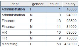
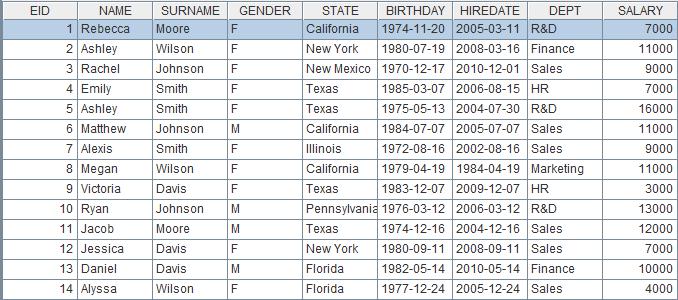
Now we want to pay attention to the gender proportion of the “good” salespersons that are computed out, that is, how many males and females there are respectively. Generally, the gender information is recorded in the employee table but not in the performance table, and it is simplified as follows:

We have already computed out the name list of “good” salespersons, and the relatively natural idea is to seek out their genders from the employee table using name list, and count the number. But in SQL, it is necessary to use join operation to get information across tables . In this way, following the initial result, SQL will be written as:

select employee.gender,count(*)

from employee,

( ( select top 10 sales from sales_amount where product='AC' order by amount desc )

intersect

( select top 10 sales from sales_amount where product='TV' order by amount desc ) ) A

where A.sales=employee.name

group by employee.gender

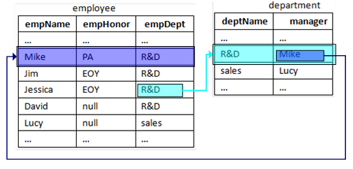
With only an associated table more, it is made so over-elaborate and in reality there are rather more cross-table storages and they are often multi-layered. For example, for salespersons, there are departments where there are managers, and now we want to know by which managers these “good” salespersons are managed. Then there are three table joins, and it is indeed no easy job to write clear where and group in this computation.

This is just the fourth important disadvantage of SQL as we want to say: Lack of object reference, in relational algebra, the relations between objects completely depends on foreign key. This not only makes the efficiency very low in looking for relation, but also makes it impossible to directly treat the record pointed by foreign key as the attribute of primary record . Try thinking, can the above statement be written as this:

select sales.gender,count(*)

from (…) // …is the SQL computing the “good” salespersons above

group by sales.gender

Evidently, this statement is not only clearer, and at the same time, the computation will also be more efficient (without join computation).

We have analyzed, through a simple example, the four important difficulties of SQL. We believe this is just the main reason why SQL fails to reach the original intention of its invention. The process of solving business problem based on a kind of computation system is in fact the process of translating business problems into formalized computation syntax (similar to the case in which a pupil solves application problem, translates the problem into formalized four arithmetic operations). Before overcoming these difficulties, SQL model system rather does not comply with people’s natural thinking habit, causing great barriers in translating problems, making it very difficult for SQL to be applied, on a large scale, in data computation for business problems.

For still another example which is easily understood by programmer, use SQL as data computation, which is similar to the case in which assembly language is used to complete four arithmetic operations. We very easily write out the calculation expression such as 3+5*7, but to use assembly language (take X86 as the example), it needs to be written as

mov ax,3

mov bx,5

mul bx,7

add ax,bx

In either writing or reading, such code is far inferior to 3+5*7 (it will be more troublesome if we come across decimal). Though it cannot be regarded as a big problem to a skilled programmer, to most people, however, this kind of writing is too hard to understand. In this sense, FORTRAN is really a great invention.